ESTIMATION OF LYAPUNOV SPECTRA FROM A TIME SERIES

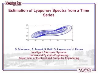
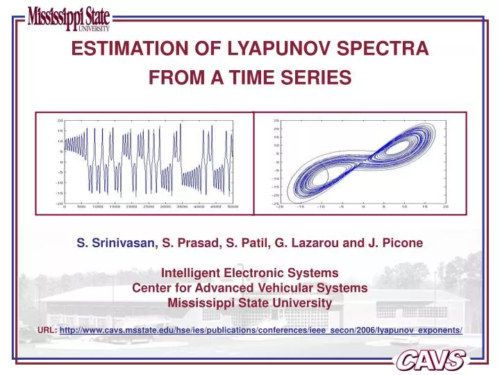
1. ESTIMATION OF LYAPUNOV SPECTRAFROM A TIME SERIES S. Srinivasan, S. Prasad, S. Patil, G. Lazarou and J. Picone Intelligent Electronic Systems Center for Advanced Vehicular Systems Mississippi State University URL: http://www.cavs.msstate.edu/hse/ies/publications/conferences/ieee_secon/2006/lyapunov_exponents/

2. Motivation • Analysis of chaotic signals: • Reconstruction a phase-space from a scalar observable • Lyapunov exponents as a tool to analyze chaos • Lyapunov spectra of chaotic and non-chaotic time series • Optimize parameters of Lyapunov spectra estimation

3. Definitions • A deterministic signal or system: every event is the result of preceding events and actions; hence predictable completely • Stochastic noise: signal that is not deterministic, i.e., inherently unpredictable • A chaotic signal or system: sensitive to initial conditions (Butterfly Effect) • Chaos says: predictability holds only in principle, hence chaotic signals are also called deterministic noise. • Dimension of a system: number degrees of freedom possessed by the system • Deterministic Chaos or Stochastic Noise? • Both have continuous power spectra (and not easily distinguishable) • Noise is infinite-dimensional. • Chaotic signals are finite dimensional, but dimension no longer associated with number of independent frequencies, but a statistical feature related to both temporal evolution and geometric aspect (self-similar structure of the attractor)

4. Power Spectrum of a Lorentz Signal • Power spectra of chaotic signals are continuous, though the system is finite dimensional. For example, the power spectrum of a 3-dimensional chaotic Lorentz signal is shown below. Stochastic systems have similar spectra even though they are infinite dimensional.

5. Attractors for Dynamical Systems • System Attractor: Trajectories approach a limit with increasing time, irrespective of the initial conditions within a region • Basin of Attraction: Set of initial conditions converging to a particular attractor • Attractors: Non-chaotic (point, limit cycle or torus),or chaotic (strange attactors) • Example: point and limit cycle attractors of a logistic map (a discrete nonlinear chaotic map)

6. Strange Attractors • Strange Attractors: attractors whose shapes are neither points nor limit cycles. They typically have a fractal structure (i.e., they have dimensions that are not integers but fractional) • Example: a Lorentz system with parameters

7. Characterizing Chaos • Exploit geometrical (self-similar structure) aspects of an attractor or the temporal evolution for system characterization • Geometry of a Strange Attractor: • Most strange attractors show a similar structure at various scales, i.e., parts are similar to the whole. • Fractal dimensions can be used to quantify this self-similarity. • e.g., Hausdorff, correlation dimensions. • Temporal Aspect of Chaos: • Characteristic exponents or Lyapunov Exponents (LE’s) - captures rate of divergence (or convergence) of nearby trajectories; • Also Correlation Entropy captures similar information. • Any characterization presupposes that phase-space is available. • What if only one scalar time series measurement of the system (and not its actual phase space) is available?

8. Reconstructed Phase Space (RPS): Embedding • Embedding: A mapping from an one-dimensional signal to an m-dimensional signal • Taken’s Theorem: • Can reconstruct a phase space “equivalent” to the original phase space by embedding with m ≥ 2d+1 (d is the system dimension) • Embedding Dimension: a theoretically sufficient bound; in practice, embedding with a smaller dimension is adequate. • Equivalence: • means the system invariants characterizing the attractor are the same • does not mean reconstructed phase space (RPS) is exactly the same as original phase space • RPS Construction: techniques include differential embedding, integral embedding, time delay embedding, and SVD embedding

9. Reconstructed Phase Space (RPS): Time Delay Embedding • Uses delayed copies of the original time series as components of RPS to form a matrix • m: embedding dimension, : delay parameter • Each row of the matrix is a point in the RPS

10. Reconstructed Phase Space (RPS) Time Delay Embedding of a Lorentz time series

11. Reconstructed Phase Space (RPS): Time Delay Embedding • Setting very small delay value: leads to highly correlated vector elements, concentrated around the diagonal in embedding space. Structure perpendicular to the diagonal not captured adequately. • Setting very large delay value: leads elements of the vector to behave as if they are independent. Evolutionary information in the system is lost. • Quantitative tools for fixing delay: plots of autocorrelation and auto-mutual information are useful guides. • Advantages: easy to compute; the attractor structure is not distorted since no extra processing is done on it. • Disadvantages: choice of delay parameter value is not obvious; leads to poor RPS in presence of noise.

12. Reconstructed Phase Space (RPS): SVD-based Embedding • Works in two stages: • Delay embed, with one sample delay, to a dimension larger than twice the actual embedding dimension • Reduce this matrix using SVD to finally have number of columns equal to embedding dimension. • (SVD-based matrix reduction is done by projecting each row onto only the first few eigenvectors and then reconstructing it to a lower-dimensional space) • SVD window size: dimension of time delayed embedded matrix over which SVD operates • Advantages: No delay parameter value to be set; more robust to noise due to SVD stage • Disadvantages: Noise reducing property of SVD may also distort the attractor properties

13. Reconstructed Phase Space (RPS): Reconstruction Attractor reconstruction using SVD embedding (for a Lorentz system)

14. Lyapunov Exponents • Quantifies separation in time between trajectories, assuming rate of growth (or decay) is exponential in time, as: • where J is the Jacobian matrix at point p. • Captures sensitivity to initial conditions. • Analyzes separation in time of two trajectories with close initial points • where is the system’s evolution function.

15. Lyapunov Exponents – Some Properties • m-dimensional system has m LE’s • LE is a measure averaged over the whole attractor • Sum of first k LE’s: rate of growth of k-dimensional Euclidean volume element • Bounded attractor: Sum of all LEs equals zero (conservative) or negative (dissipative) • Zero exponents indicate periodic attractor (limit cycle) or a flow • Negative exponents pull points in the basin of attraction to the attractor • Positive exponents indicate divergence: signature for existence of chaos

16. Lyapunov Exponents: Computation • Embed time series to form RPS matrix. Rows represent points in phase space • Take first point as center • Form neighborhood matrix, each row obtained by subtracting a neighbor from the centre • Find evolution of each neighbor and form the evolved neighborhood matrix by subtracting each evolved neighbor from the evolved centre • Compute trajectory matrix at the center by multiplying pseudo-inverse of neighborhood matrix with evolved neighborhood matrix • Advance center to a new point and go to step 3, averaging the trajectory matrix in each iteration • The LEs are given by the average of the eigenvalues from each R matrix. Direct averaging has numerical issues, hence an iterative QR decomposition method (treppen-iteration) is used.

17. Input time series Embed the data Locate nearest points Form neighborhood Evolve “a” steps Locate nearest points Form neighborhood Calculate trajectory martix Perform QR decomposition o Locate nearest points Calculate exponents from R Evolve center • Lyapunov Exponents: Computation Flowchart

18. Experimental Design • Three systems tested : two chaotic (Lorentz and Rossler) and one non-chaotic (sine signal) • Two test conditions: clean and noisy (10 dB white noise) • Lorentz system: • Parameters: • Expected LEs: (+1.37, 0, -22.37) • Rossler system: • Parameters: a = 0.15, b = 0.2, c = 10 • Expected LEs: (0.090, 0.00, -9.8) • Sine Signal: • Parameters: Freq=1Hz, Samp freq=16Hz, Amp=1 • Expected LEs: (0.00, 0.00, -1.85)

19. Experimental Design • Experiments performed to optimize parameters of estimation algorithm • 30,000 points were generated for each series in both the conditions • 5,000 iterations (or the number of evolution steps) were used for averaging using QR treppen-iteration • Variation of LEs with SVD window size and number of nearest neighbors • Varied number of neighbors with SVD window size: 15 for clean data; 50 for noisy data • Varied SVD window size with number of neighbors: 15 for clean data; 50 for noisy data

20. Experimental Results Lyapunov Exponents (LEs) for a Lorentz System • For clean data: Positive and zero exponents are almost constant at the expected values • For noisy data: Positive and zero exponents converge to the expected value for SVD window size about 50 and number of neighbors also about 50 • Negative LE estimation: not reliable

21. Experimental Results Lyapunov Exponents (LEs)for a Rossler System • For clean data: Positive and zero exponents are almost constant at the expected values • For noisy data: Positive and zero exponents converge to the expected value for SVD window size about 60 and number of neighbors also about 50 • Negative LE estimation: not reliable

22. Experimental Results Lyapunov Exponents (LEs)for Sine Signal • For clean data: Positive and zero exponents are almost constant at the expected values • For clean data: Positive and zero exponents converge to the expected value for SVD window size about 40 and number of neighbors also about 30 • Negative LE estimation: not reliable

23. Summary and Future Work • LEs are useful in quantifying how chaotic a system is. • SVD embedding helps reconstructing phase spaces in noisy conditions. • Parameters of the LE computation algorithm are optimized experimentally to get reliable estimates. • Both the positive and zero LE’s are estimated near the actual values using optimized parameters. • Negative LE estimation is unreliable (but this is of little concern in chaotic systems). • The code for LE estimation is publicly available. • Our future work will be to apply Lyapunov exponents to model nonlinearities in speech for better automatic speech recognition.

24. Pattern Recognition Applet: compare popular linear and nonlinear algorithms on standard or custom data sets • Speech Recognition Toolkits: a state of the art ASR toolkit for testing the efficacy of these algorithms on recognition tasks • Foundation Classes: generic C++ implementations of many popular statistical modeling approaches • Resources

25. References • J. P. Eckmann and D. Ruelle, “Ergodic Theory of Chaos and Strange Attractors,” Reviews of Modern Physics, vol. 57, pp. 617‑656, July 1985. • M. Banbrook, “Nonlinear analysis of speech from a synthesis perspective,” PhD Thesis, The University of Edinburgh, Edinburgh, UK, 1996. • E. Ott, T. Sauer, J. A. Yorke, Coping with chaos, Wiley Interscience, New York, New York, USA, 1994. • M. Sano and Y. Sawada, “Measurement of the Lyapunov Spectrum from a Chaotic Time Series,” Physical Review Letters, vol. 55, pp. 1082-1085, 1985. • G. Ushaw, “Sigma delta modulation of a chaotic signal,” PhD Thesis, The University of Edinburgh, Edinburgh, UK, 1996.