Download
1 / 32
320 likes | 456 Views
Geometric Interpretation of Linear Programs. Chris Osborn, Alan Ray, Carl Bussema, and Chad Meiners 16 March 2005. Feasibility in 3-Space. Five total constraints; therefore 5 faces to the polyhedron. Simplex Illustrated: Initial Dictionary. Current solution: x 1 = 0 x 2 = 0 x 3 = 0

E N D
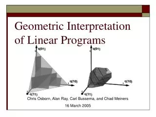
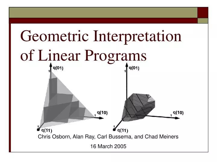
Geometric Interpretation of Linear Programs Chris Osborn, Alan Ray, Carl Bussema, and Chad Meiners 16 March 2005
Feasibility in 3-Space • Five total constraints; therefore 5 faces to the polyhedron
Simplex Illustrated: Initial Dictionary Current solution: x1 = 0 x2 = 0 x3 = 0 z=3x1+2x2+5x3=0
Simplex Illustrated: First Pivot Current solution: x1 = 0 x2 = 0 x3 = 5 z=3x1+2x2+5x3=25
Simplex Illustrated: Second Pivot Current solution: x1 = 2 x2 = 0 x3 = 5 z=3x1+2x2+5x3=31
Simplex Illustrated: Final Pivot Final solution (optimal): x1 = 0 x2 = 4 x3 = 5 z=3x1+2x2+5x3=33
Simplex Review and Analysis • Simplex pivoting represents traveling along polyhedron edges • Each vertex reached tightens one constraint (and if needed, loosens another) • May take a longer path to reach final vertex than needed
The Graphic Method • Use geometry to quickly solve LP problems in 2 variables • Plot all restrictions in 2D plane (x1, x2) • Result plus axes forms polyhedron • Region of feasible solutions • Draw any line with same slope as objective function through polyhedron • “Move” line until leaving feasible region • i.e., Find parallel tangent
Graphic Method Example:Step 1: Plot Boundary Conditions max 5x1 + 4x2 subject to: x1 – 3x2 ≤ 3 2x1 + 3x2 ≤ 12 -2x1 + 7x2 ≤ 21 x1,x2 ≥ 0
Graphic Method Example:Step 2: Determine Feasibility max 5x1 + 4x2 subject to: x1 – 3x2 ≤ 3 2x1 + 3x2 ≤ 12 -2x1 + 7x2 ≤ 21 x1,x2 ≥ 0 Based only on this, where might the optimal solution be?
Graphic Method Example:Step 3: Plot Objective = c max 5x1 + 4x2 subject to: x1 – 3x2 ≤ 3 2x1 + 3x2 ≤ 12 -2x1 + 7x2 ≤ 21 x1,x2 ≥ 0
Graphic Method Example:Step 4: Find Parallel Tangent max 5x1 + 4x2 subject to: x1 – 3x2 ≤ 3 2x1 + 3x2 ≤ 12 -2x1 + 7x2 ≤ 21 x1,x2 ≥ 0 Optimal solution: x1=5, x2=2/3, z=83/3
Second Graphic Method Example max 4x1 + 6x2 subject to: x1 – 3x2 ≤ 3 2x1 + 3x2 ≤ 12 -2x1 + 7x2 ≤ 21 x1,x2 ≥ 0 Same constraints; new objective. What changes?
Second Graphic Method Example:No Tangent Exists max 4x1 + 6x2 subject to: x1 – 3x2 ≤ 3 2x1 + 3x2 ≤ 12 -2x1 + 7x2 ≤ 21 x1,x2 ≥ 0 Optimal solution: 1.05 ≤ x1 ≤ 5, 2x1 + 3x2 = 12, z=24
Consider earlier problem:max 5x1 + 4x2 subject to: x1 – 3x2 ≤ 3 2x1 + 3x2 ≤ 12 -2x1 + 7x2 ≤ 21 x1,x2 ≥ 0 Optimal: x1*=5, x2*=2/3 Prove optimal if equal to corresponding dual solution min 3y1 + 12y2 + 21y3 subject to: y1 + 2y2 – 2y3 ≥ 5 -3y1 + 3y2 + 7y3 ≥ 4 y1, y2 ≥ 0 Geometric Interpretation of Duality
Geometric Duality Continued • Think of dual variables as coefficients for primal constraints (α = y1, = y2, = y3):(α) (x1 – 3x2) ≤ (α) 3() (2x1 + 3x2) ≤ () 12() (-2x1 + 7x2) ≤ () 21 • Resulting sum is linear combination:(α+2-2)x1 + (-3α+3+7)x2 ≤ 3α+12+21 • We can graph this for various choices of α, , and
Geometric Duality: Linear Combinations Graphed (α+2-2)x1 + (-3α+3+7)x2 ≤ 3α+12+21 • Three examples shown • α = = 1, = 0 • α = = = 1 • α = 0, = = 1 • Pink line is parallel tangent • Notice: primal solution two vertices away from origin • Two constraints matter; third irrelevant here. • Duality implication: = 0
Geometric Duality Graphed Again (α+2)x1 + (-3α+3)x2 ≤ 3α+12 • Gives a line always passing through (5,2/3), the primal solution • If primal solution optimal, there must exist some α, such that resulting line matches parallel tangent. Why? • Duality theorem guarantees
Convex Set and Hulls • Convex Sets • Convex Hulls • Applying LP Theorem to Convex Sets and Hulls
Convex Sets S1 • Two of these sets are not like the others • S1 and S4 are convex • S2 and S3 are not • A set S Rn is convex iff • Given a,b S • For all 0 ≤t≤ 1 • ta + (1-t)bS S2 S3 S4
Property of Convex Sets • The intersection of two convex sets results in a convex set • Every set has a minimal convex set that contains it
Convex Hulls • Given a set S Rn • Convex Hull H • Contains S • Is convex • Is contained by all convex sets containing S (i.e. it is minimal)
z1 z z3 z2 Convex Hulls as Linear Equations • Given a set S Rn • For each point z in H • There are k points z1,…,zk in S • positive variables t1,…,tk • Such that z = ti zi 1 = ti
LP Theorem • If a system of m linear equations has a nonnegative solution, then it has a solution with at most m positive variables • So given v=1…n aivxv = b (for i = 1…m) xv≥ 0 • At most m of the variables x1…xn are positive
z1 z z3 z2 Implications Upon Convex Hulls • For a space S Rn • We have at most n+1 points that define a hull point • So for R2, every point z in H is defined by at most 3 points in S • Why? • Hull points are represented by n+1 linear equations • Thus we have at most n+1 positive scaling variables ti
Some More Observations • Every half-space is convex • Every polyhedron is convex • The convex hull of a finite set of points is a polyhedron
LP Theorem • Every unsolvable system of linear inequalities for n variables contains a unsolvable subsystem of at most n+1 inequalities • We use this theorem for the common point theorem
Common Point Theorem • Let F be a finite family of at least n + 1 convex sets in Rn • Such that every n+1 sets in F have a point in common • All sets in F have a point in common
Common Point Theorem (continued) • Note that we can’t make guarantees without every n+1 sets in F having a point in common
Common Point Theorem (Why) • The intersection of each n+1 sets is a system of n+1 linear inequialities • Therefore the whole system cannot have an unsolvable subsystem of n+1 linear inequalities • Thus we have a point in common for the family of convex sets
Separation Theorem for Polyhedra • For every pair of disjoint polyhedra • There exists a pair of disjoint half-spaces • Such that each half-space contains a polyhedron
Conclusions • Geometry useful for: • Understanding properties of linear programs • Solving (some) linear programs • Modeling linear programs visually • And geometric problems can be modeled with linear programs • Questions?