Download
1 / 32
330 likes | 460 Views
Welcome to CSE 599. Instructor: Rajesh Rao (rao@cs.washington.edu) TA: Aaron Shon (aaron@cs.washington.edu) Class web page http://www.cs.washington.edu/education/courses/599/CurrentQtr/ Add yourself to the mailing list see the web page Today’s lecture: Course Introduction

E N D
Welcome to CSE 599 • Instructor: Rajesh Rao (rao@cs.washington.edu) • TA: Aaron Shon (aaron@cs.washington.edu) • Class web page • http://www.cs.washington.edu/education/courses/599/CurrentQtr/ • Add yourself to the mailing list see the web page • Today’s lecture: • Course Introduction • What is Computation? • History of Computing • Theoretical Foundations: Part I
Course goals • To examine the future of computing • Moore's law will certainly end. What are the alternatives? • Biologically-inspired and quantum computing • To broaden your perspectives on the fundamental aspects of computation • To give you sufficient exposure to • understand the premises of alternative computing paradigms • allow you to pursue these topics further • What we will not accomplish • Mastery of any specific field
What we will cover • Background topics • Theoretical foundations of computer science • Silicon technology and digital computer organization • Information theory and thermodynamics • DNA computing • Using DNA-binding properties to solve computationally hard problems • Neural computing • Computation in animal brains and in artificial neural networks • Quantum computing • Using quantum superposition for massively parallel computation
Sequence of Lecture Topics • Theoretical Foundations of Computer Science (Jan 4 & 11) • Silicon Technology and Digital Computing (Jan 18, including a guest lecture by Chris Diorio, UW) • DNA Computing (Jan 25, including a guest lecture by Anne Condon, UBC) • Neural Computing (Feb 1 & 8) • Information Theory and Thermodynamics (Feb 15) • Quantum Computing (Feb 22, including a guest lecture by Dan Simon, Microsoft Research)
Grading, homework, and other logistics • Grading: Homeworks 50%, Mini-Project 50% • Homework assignments will be handed out on the day of the lecture related to the homework (see Course web page) • Homeworks are due at the beginning of class on the specified due date (see Course web page) • Pick a mini-project related to a course topic (project ideas will appear on Course web…or come up with your own!) • Project presentations: beginning of March • Project reports due: finals week (Mar 12-15)
OK, enough about the course.Let’s get started… What is computation? What does it mean to “compute” something? What is a computer?
What is a computer? • Consider the following: • A coffee filter • A wheat threshing machine • A handful of spaghetti • Can these be viewed as computers??
Yes, if you can find a useful mapping… • For example, consider the handful of spaghetti • Suppose you want to sort 100 numbers • Take 100 sticks of spaghetti and cut them to the length of your numbers • Hold the spaghetti sticks and align their bottom ends on a table • Pick out the tallest stick, then the next tallest, and so on… • You have just sorted your 100 numbers using a spaghetti “computer”!
So, what is a computer? • A working definition: • A computer is a physical system whose: • physical states can be seen as representing elements of another system of interest • transitions between states can be seen as operations on these elements • Three basic steps: • Input data is coded into a form appropriate for physical system • Physical system shifts into a new state • Output state of system is decoded to extract results of computation • Consider these 3 steps for our spaghetti computer example. Also holds for silicon, DNA, neural, and quantum computers.
If computers can have such varied substrates, how did we end up with silicon-based digital computers on our desks (rather than, say, organic, spaghetti-manipulating analog computers)? Answer: Because of a convergence of theoretical and practical ideas in the history of computing…
A Brief History of Computing • The early years: • Mapping numbers to objects (e.g. stones) • Adding and subtracting by manipulation • Stonehenge (~ 2800 BC) – a prehistoric computer of solar eclipses? • The first personal “calculator” – the abacus (a mnemonic aid based on place-value notation)
Early pioneers in software and hardware… • Muhammad ibn Musa Al’Khorizmi • Proposed the concept of an “algorithm” as a written process that achieves a certain goal when executed • Published first book on “software” (12th century) • Blaise Pascal • Built a mechanical adding machine in 1642 • Numbers mapped to dials and gears • Based on differential transmission via gears of different sizes
The middle ages (1800-1900)… • First software-based controller (1801): • J.-M. Jacquard’s Automatic Loom • Control program written on punched cards • Babbage’s ideas for steam-powered computers • Difference Engine (1822) for computing mathematical tables • Analytical Engine (1833) for general computation (introduced conditionals) • Both were never constructed
Punched cards and digital computing… • Used by Hollerith to input data to his “Tabulating machine” for tabulating and counting census information (1890) • Perforated strips of discarded movie film used by Zuse to control the first programmable digital computers (Z1-Z3)
The digital computer revolution • ~1850: George Boole invents Boolean algebra • Maps logical propositions to symbols • Allows us to manipulate logic statements using mathematics • 1936: Alan Turing develops the formalism of Turing Machines • 1945: John von Neumann proposes the stored computer program concept • 1946: ENIAC: 18,000 tubes, several hundred multiplications per minute • 1947: Shockley, Brattain, and Bardeen invent the transistor • 1956: Harris introduces the first logic gate • 1972: Intel introduces the 4004 microprocessor • Present: <0.2 m feature sizes; processors with >20-million transistors
What is computable? • We have examined how developments in theory and technology paved the way for the digital computers we use today • A key concept that allowed general purpose computing: the stored program idea • Theoretical roots: Turing machines, Machines simulating other machines, Universal Turing Machines • Church-Turing Thesis: The Turing machine is equivalent in computational ability to any general mathematical device for computation, including digital computers. • Important Result: There exist functions that are not computable by any computational device
5 minute break…. (Next: Theoretical foundations of computing)
Introduction • We asked what computation was - now we’ll try to answer the question “what is computable?” • These results about computability are fundamental. • They apply regardless of the machine • But they don’t answer all of our questions • One of the major contributions of theoretical CS: negative results
Abstract Models of Computation • We want to answer fundamental questions: • What can we do in a reasonable amount of time? • What can we do in a reasonable amount of space? • What can we do at all? • AMAZING result-- some things are not computable!
A First Model for Computation: Automata • Chalkboard Example…(automata for Parity, from Feynman text, chapter 3)
Languages • A language is some set of strings • The language of a FA is the set of strings the FA recognizes • In the parity example, we can write • L = 0* (1 0* 1)* 0*
In-Class Exercise • Design a Finite Automata that accepts strings where the number of 1’s AND the number of 0’s is even…
Limitations of DFA’s • Cannot recognize some languages e.g. balanced parens, 0n1n • Only a finite number of states, so it can’t count. • We can actually characterize what languages DFA’s recognize exactly • Called regular languages
DFA’s vs. Computers • Technically, computers are DFA’s • BUT- we think they can answer questions like 0n1n • They actually can’t-- what if n was 10100? • We think of computers as storing numbers, instead of moving to a state which represents storing that number, but the general notion is the same
Turing Machine • Equivalent to a finite automaton that has an unbounded tape • Has a head which can move left or right, as well as write symbols on the tape • The TM is aware of what the head is looking at • Can defined as a “program” or list of quintuples: • (current state, current symbol on tape) to (next state, new symbol to write, direction of head movement), or • (q, s, q’, s’, d) • There exists an initial state q0 and a set of halting states
An Example of a Turing Machine • A Turing Machine for checking if parentheses are balanced (from Feynman text, chapter 3) • E.g. Tape contains …E()E…, or …E(()(E…, or …E((()()))E…
Exercise on Turing Machines… • Design a Turing machine that multiplies two unary numbers • Example: Tape contains …111X11… Answer should be: …111111… • For a complete solution, see the handout (chapter 28 of The Turing Omnibus by Dewdney)
Solution Sketch • A TM that multiplies unary numbers • Example: Tape contains …111X11… Answer is: …111111… • Pseudocode: On input string w: • Write a * to the left of the input to separate the output from input • For each 1 occurring after the X: • For each 1 occurring before the X: Write a 1 in the leftmost blank cell of the tape beyond the * End for End for • Erase the * and all symbols to the right of it • Halt
Alternate Models of TMs • Multitape TMs • equivalent to ordinary TMs • TMs with Rectangular Grids • TM that can jump to arbitrary locations on the tape • Nondeterministic TMs • equivalent to TM in terms of computability • Will play an important role in the next class
The stage is set to tackle the big questions… • What functions are computable? • We can now ask: Are there functions that a Turing machine cannot compute? • What functions are tractable? • For what type of problems do fast and efficient algorithms exist? • By efficient, we mean time- and space-efficient • This will then allow us to look at: Problems that are hard to solve on conventional computers but can be solved more efficiently using alternative computing methods such as DNA, neural, or Quantum Computing
Next week: Theoretical Foundations (Part II) • Turing machines that simulate other Turing machines • Universal Turing machines • Halting problem and Undecidability • Computational Complexity: Time and Space Efficiency • P, NP, and NP-complete problems Read the handout given today and Feynman chapters 1-3… Have a great weekend!