Download
1 / 22
220 likes | 367 Views
Lecture 21: Trends, Seasonality & Polynomial Regression. April 7 th 2014. Question. Given the following regression, which of the follow is true B2 is the partial slope of Age, holding Female constant B2 is the partial slope of Age, when Female =0 (i.e., males)

E N D
Lecture 21: Trends, Seasonality & Polynomial Regression April 7th 2014
Question Given the following regression, which of the follow is true • B2 is the partial slope of Age, holding Female constant • B2 is the partial slope of Age, when Female =0 (i.e., males) • B1 is the partial slope of Female, holding Age constant. • None of the above • More than one of the above.
Administrative • Quiz 5 next Monday • Exam 3 two weeks from today. • Problem Set 8 due Thursday at noon. • Exam 2 results: • Soon… (this week) It’s taking a long time to grade.
Last time • Moving average and Exponential smoothing
Simple Exp Smoothing • We’ll refer to the level of a series at time t as Lt for a given smoothing constant α: • A the future forecast for any time t+k • Note • Levels are defined recursively; L1 = Y1 • All future forecasts are just the last level (or smoothed) value. • NO TREND modeled.
Simple Exp Smoothing • From the previous equations it follows that the predicted level at any time t is just a function of the previous observed amounts: • What value of α should you use? • Eh… hard to stay. 0.1? 0.2? • Lower is smoother. (the weights in the book w, are 1-α and hence larger w produce smoother forecasts). • You can let StatTools optimize α to minimize RSME • Keep in mind that this could run the risk of overfitting your data
Drawbacks. • Simple moving and exponentially weighted averages don’t do so well when there is a trend in the data:
Holt’s Method Modeling a Trend: • If there is an obvious trend in the data, we might want to model it. A second method is due to Holt: Where Tt is the trend term at time t with a trend smoothing constant
Holt Example • Using the HouseSales.xlsx data, compare the forecast using a simple exponentially weighted average without a trend and Holt’s method (which includes a trend component). Which of the following is the best answer (alpha =.2): • The MAPE using Holt’s method is 1.88% points less than using the simple exponentially weighted average • The RMSE for the forecast using Holt’s method is 69.91 • The RMSE for the Holt’s method is worse than the simple average. • More than one of the above
Manually deseasonalizing data Deseasonalize data using the ratio-to-moving average method: • Start with July, calculate the moving average from previous January through the future December (12 months) • This MA from is centered from mid June through mid July • Calculate a 2nd moving average from the previous February through the future January (12 months) • This is centered around the mid July through mid August. • Average (1) and (2) to get a smoothed estimate for July. • Divide the actual July amount by (3) to get a seasonal index for that July • Average (or take the median) of all the July indexes • Repeat for each month • All of the indexes for a calendar year should add to 12. If they don’t multiply them by the constant = 12 / (sum of indexes)
Deseasonalizing • Thankfully StatTools can take care of seasonality in the forecasting methods we discussed last time • Moving and Exponentially weighted Averages • Holt’s method • Example with SoftDrinkSales.xls
Winters’ Method 3 types of exponential smoothing: • Simple: appropriate for a series with no trend or seasonality • Holt’s method: for a series with a trend but no seasonality. • Winters’ method: for seasonality & possible trend. • 3 parameters: α, β, γ and M seasons
Validating the Forecasts Holdouts: Specifies the number of observations to "hold out", or not use in, the forecasting model. • You can choose to use all of the observations for estimating the forecasting model (0 Holdouts), • Or hold out a few for validation. Then the model is estimated from the observations not held out, and it is used to forecast the held-out observations
Winter’s Method Example Using the SoftDrinkSales.xls data, hold out 2 years of data. Which method produces the lowest RMSE during the holdout period? • Simple Exponential • Holt’s method • Winter’s method • I’m very tired and want to go home.
Regression Forecasting Models Simple regression of trend: • Use time as an independent variable • Seasonality with Regression: • Use dummy variables to represent the seasons (quarters, etc):
Seasonality • Seasonality with Regression: • Use dummy variables to represent the seasons (quarters, etc):
Seasonality • By including dummy variables for the time components, you’re modeling the seasonality directly, • But you’re also assuming it will only be a constant intercept shift from the other seasons. • Sometimes this is fine. Sometimes it’s not • Examples? • difference between additive vs multiplicative seasonality
Non-linear Regression Polynomial regression: • Uses powers of time as independent variables • Example of a 4th degree polynomial:
Polynomial Regression • Higher orders allow for better fits of the observed data: • Look at the R2 below:
Polynomial Regression • But… Outside of the observed data, very bad things can happen: • In general, avoid fitting models of high order polynomials
Polynomial Regression Sidebar: • You can fit a polynomial regression for non-time-series data. • i.e., you can include things like Income3 or Income4 but we’ve avoided higher order polynomials it in the class. • We’ve done things like Income1/2 or Income-2 • Sometimes it’s completely fine to fit a higher order polynomial regression equation, but ask yourself why. • Realize your regression model is probably “wrong” to some extent anyway. • What we’re often after is a good generalizable model. Don’t make the model overly complicated.
Next Time • Autoregressive Models • AR(1) and AR(p)