Download
1 / 48
540 likes | 810 Views
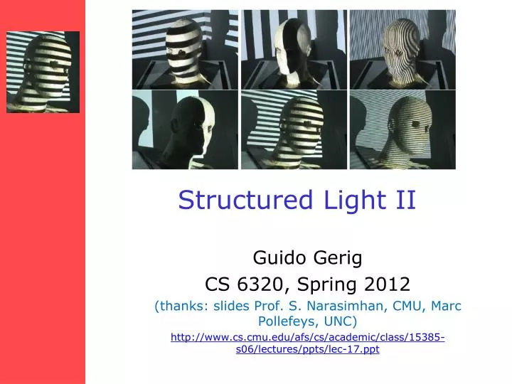
Structured Light II. Guido Gerig CS 6320, Spring 2012 (thanks: slides Prof. S. Narasimhan , CMU, Marc Pollefeys , UNC) http://www.cs.cmu.edu/afs/cs/academic/class/15385-s06/lectures/ppts/lec-17.ppt. Faster Acquisition?. Project multiple stripes simultaneously

E N D
Structured Light II Guido Gerig CS 6320, Spring 2012 (thanks: slides Prof. S. Narasimhan, CMU, Marc Pollefeys, UNC) http://www.cs.cmu.edu/afs/cs/academic/class/15385-s06/lectures/ppts/lec-17.ppt
Faster Acquisition? • Project multiple stripes simultaneously • Correspondence problem: which stripe is which? • Common types of patterns: • Binary coded light striping • Gray/color coded light striping
Static Light Pattern Projection • Project a pattern of stripes into the scene to reduce the total number of images required to reconstruct the scene. • Each stripe/line represents a specific angle α of the light plane. • Problem: How to uniquely identify light stripes in the camera image when several are simultaneously projected into the scene.
Time-Coded Light Patterns • Assign each stripe a unique illumination codeover time [Posdamer 82] • #stripes = mn : m gray levels, n images Time Space
Binary Coding: Bit Plane Stack • Assign each stripe a unique illumination codeover time [Posdamer 82] Time Space
Binary Encoded Light Stripes • Set of light planes are projected into the scene • Individual light planes are indexed by an encoding scheme for the light patterns • Obtained images form a bit-plane stack • Bit-plane stack is used to uniquely address the light plane corresponding to every image point http://www.david-laserscanner.com/
Time Multiplexing • A set of patterns are successively projected onto the measuring surface, codeword for a given pixel is formed by a sequence of patterns. • Themostcommonstructure of thepatternsis a sequence of stripesincreasingitswidthbythe time single-axis encoding • Advantages: • highresolution a lot of 3D points • High accuracy (order of m) • Robustnessagainstcolorfulobjectssincebinarypatterns can be used • Drawbacks: • Staticobjectsonly • Largenumber of patterns Projected over time Example: 5 binary-encoded patterns which allows the measuring surface to be divided in 32 sub-regions
Binary Coding Example: 7 binary patterns proposed by Posdamer & Altschuler Projected over time … Pattern 3 Pattern 2 Pattern 1 Codeword of this píxel: 1010010 identifies the corresponding pattern stripe
Binary Coding (II) • Binary coding • Only two illumination levels are commonly used, which are coded as 0 and 1. • Gray code can be used for robustness (adjacent stripes must only differ in 1 bit) • Everyencodedpointisidentifiedbythesequence of intensitiesthatitreceives • n patternsmust be projected in ordertoencode 2nstripes • Advantages • Easy to segment the image patterns • Need a large number of patterns to be projected
Gray Code • Frank Gray (-> name of coding sequence) • Code of neighboring projector pixels only differ by 1bit, possibility of error correction!
Concept Gray Code(adjacent stripes must only differ in 1 bit)
N-ary codes • Reduce the number of patterns by increasing the number of intensity levels used to encode the stripes. • Multi grey levels instead of binary • Multilevel gray code based on color. • Alphabet of m symbols encodes mnstripes 3 patterns based on a n-ary code of 4 grey levels (Horn & Kiryati) 64 encoded stripes
Gray Code + Phase Shifting (I) • A sequence of binary patterns (Gray encoded) are projected in order to divide the object in regions Example: three binary patterns divide the object in 8 regions Without the binary patterns we would not be able to distinguish among all the projected slits • An additional periodical pattern is projected • The periodical pattern is projected several times by shifting it in one direction in order to increase the resolution of the system similar to a laser scanner Every slit always falls in the same region Gühring’s line-shift technique
Phase Shift Method (Guehring et al) • Project set of patterns • Project sin functions • Interpolation between adjacent light planes • Yields for each camera pixel corresponding strip with sub-pixel accuracy! • See Videometrics01-Guehring-4309-24.pdf for details
Source: http://www.igp.ethz.ch/photogrammetry/education/lehrveranstaltungen/MachineVisionFS2011/coursematerial/MV-SS2011-structured.pdf
(or light stripe) (or light stripes)
Coded structured light • Correspondence without need for geometrical constraints • For dense correspondence, we need many light planes: • Move the projection device • Project many stripes at once: needs encoding • Each pixel set is distinguishable by its encoding • Codewords for pixels: • Grey levels • Color • Geometrical considerations
Pattern encoding/decoding • A pattern is encodedwhen after projecting it onto a surface, a set of regions of the observed projection can be easily matched with the original pattern. Example: pattern with two-encoded-columns • The process of matching an image region with its corresponding pattern region is known as pattern decoding similar to searching correspondences • Decoding a projected pattern allows a large set of correspondences to be easily found thanks to the a priori knowledge of the light pattern Object scene Pixels in red and yellow are directly matched with the pattern columns Codification using colors
Rainbow Pattern http://cmp.felk.cvut.cz/cmp/demos/RangeAcquisition.html Assumes that the scene does not change the color of projected light.
Direct encoding with color • Every encoded point of the pattern is identified by its colour Tajima and Iwakawa rainbow pattern (the rainbow is generated with a source of white light passing through a crystal prism) T. Sato patterns capable of cancelling the object colour by projecting three shifted patterns (it can be implemented with an LCD projector if few colours are projected)
Pattern encoding/decoding • Two ways of encoding the correspondences: single and double axis codification it determines how the triangulation is calculated • Decoding the pattern means locating points in the camera image whose corresponding point in the projector pattern is a priori known Single-axis encoding Double-axis encoding Triangulation by line-to-plane intersection Triangulation by line-to-line intersection
More complex patterns Works despite complex appearances Works in real-time and on dynamic scenes • Need very few images (one or two). • But needs a more complex correspondence algorithm Zhang et al
Drawbacks: • Discontinuitiesontheobjectsurface can produce erroneouswindowdecoding (occlusionsproblem) • Thehigherthenumber of usedcolours, the more difficulttocorrectlyidentifythemwhenmeasuring non-neutral surfaces • Maximumresolutioncannot be reached • Advantages: • Movingobjectssupported • Possibilityto condense thecodificationto a uniquepattern Spatial Codification • Project a certain kind of spatial pattern so that a set of neighborhood points appears in the pattern only once. Then the codeword that labels a certain point of the pattern is obtained from a neighborhood of the point around it. • Thecodificationiscondensed in a uniquepatterninstead of multiplexingitalong time • Thesize of theneighborhood (windowsize) isproportionaltothenumber of encodedpoints and inverselyproportionaltothenumber of usedcolors • Theaim of thesetechniquesistoobtain a one-shotmeasurementsystem movingobjects can be measured
Local spatial Coherence http://www.mri.jhu.edu/~cozturk/sl.html • Medical Imaging LaboratoryDepartments of Biomedical Engineering and RadiologyJohns Hopkins University School of MedicineBaltimore, MD 21205
De Bruijn Sequences • A De Bruijn sequence(orpseudorandom sequence)of order m over an alphabet of n symbols is a circular string of length nm that contains every substring of length m exactly once (in this case the windows are one-dimensional). • 1000010111101001 • The De Bruijn sequences are used to define colored slit patterns (single axis codification) or grid patterns (double axis codification) • In order to decode a certain slit it is only necessary to identify one of the windows in which it belongs to ) can resolve occlusion problem. m=4 (window size) n=2 (alphabet symbols) Zhang et al.: 125 slits encoded with a De Bruijn sequence of 8 colors and window size of 3 slits Salvi et al.: grid of 2929 where a De Bruijn sequence of 3 colors and window size of 3 slits is used to encode the vertical and horizontal slits
M-Arrays • An m-array is the bidimensional extension of a De Bruijn sequence. Every window of wh units appears only once. The window size is related with the size of the m-array and the number of symbols used • 0 0 1 0 1 0 • 0 1 0 1 1 0 • 1 1 0 0 1 1 • 0 0 1 0 1 0 Example: binary m-array of size 46 and window size of 22 Shape primitives used to represent every symbol of the alphabet M-array proposed by Vuylsteke et al. Represented with shape primitives Morano et al. M-array represented with an array of coloured dots
Binary spatial coding http://cmp.felk.cvut.cz/cmp/demos/RangeAcquisition.html
16th transition Decoding table
De Bruijn Experimental results Gühring