Download
1 / 1
10 likes | 113 Views
The Connection Between Conceptual Model Errors and the Capabilities of Numerical Ground-Water Flow Models MARY C. HILL 1 and STEFFEN MEHL 1,2 1 U.S. GEOLOGICAL SURVEY, BOULDER, COLORADO, USA 2 DEPT. OF CIVIL, ENVIRONMENTAL & ARCHITECTURAL ENGINEERING, UNIVERSITY OF COLORADO, BOULDER.

E N D
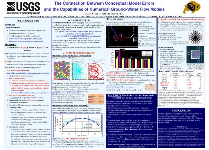
The Connection Between Conceptual Model Errors and the Capabilities of Numerical Ground-Water Flow ModelsMARY C. HILL1and STEFFEN MEHL1,2 1U.S. GEOLOGICAL SURVEY, BOULDER, COLORADO, USA 2 DEPT. OF CIVIL, ENVIRONMENTAL & ARCHITECTURAL ENGINEERING, UNIVERSITY OF COLORADO, BOULDER A CHANGING WORLD New field data methods, like tomography, reveal unprecedented subsurface detail that can support smaller scale conceptualizations. More powerful computers and software make simulating these smaller scales feasible. Are ground-water model CAPABILITIES adequate to take advantage of these opportunities? Here: Do ERRORS and LIMITATIONS in present model capabilities hold us back? Many useful analyses have been done. Here we present some we conducted using the popular and relatively mature MODFLOW ground-water model. Results are expected to apply to any discretized modeling method unless noted. 2. Scale of system features Hydraulic-conductivity field: Heterogeneity Example from Mehl and Hill (2002a) Local features: variation changes shape of flow lines, but some bulk flow and transport characteristics mimic those of a simpler model. Persistentfeatures: can be very important to transport. Need to consider data, importance to predictions, and execution time to determine what heterogeneity to explicitly represent Model features can affect conceptualization. MODFLOW’s Hydrogeologic-Unit Flow Package allows hydrogeologic units and parameters to be defined separately from model layers. Vertical grid refinement can be implemented as warranted by observations and predictions. Hydraulic-conductivity field: Anisotropy Many ground-water models are limited in their ability to represent spatially variable anisotropy. An analysis by Anderman and others (in press) using a simple 2D problem developed by John Wilson (NM Inst. of Tech.) shows: Implications: up to30% errors inlocal flows. With the new LVDA Capability, horizontal and vertical anisotropy now supported by MODFLOW, so this limitation largely resolved for this model. Finite-element models FEMWATER, SUTRA3D, FEHM, etc have even greater flexibility. Important, for example, to simulate a syncline. • INTRODUCTION • PROBLEM • Conceptual Models • Define characteristics and processes thought to be important to predictions of interest. • Provide blueprints for model development • Influenced by the capabilities, errors, and limitations of the mathematical model used? APPROACH CONSIDER ONLY SCALE ISSUES IN 3-D SYSTEMS Reasons: 3-Dimportant in all but very simple systems. Generally doable now or will be soon given modern computer capabilities. No need to compromise. SCALE issues that are spatial are important, as shown below. For numerical models, spatial scale and grid scale are interrelated. How do these issues fit into the larger picture? Red: Issues considered here. Blue: Math model abilities influence conceptual model • Interpretation(s) of system features • Scale of system features • Commonly consider scales that can be simulated • Consider scales important to purpose of model, but this can change as the model is used. Commonly subsequent analysis limited to features represented in the originally constructed model. • For both, model capabilities influence conceptual model • Scale needed for numerical accuracy • Governed by the capabilities of the model used. • Dimensionality: 1-, 2-, or 3-D? Steady or transient? • Deterministic or stochastic? • Integration with other processes, such as surface processes • Parameter values • For conceptual models, use expected values of K, etc to design a model accurate enough to be useful and tractabl eenough to calibrate. • Fundamental issue: Spatial contrasts versus smoothness (zonation or indicator kriging good for contrasts; interpolation and regularization good for smooth fields). Presently zonation most common. • Discretization method • Finite difference, finite element, analytic element, and so on. • In some situations, the solutions produced by some types of discretization contain large errors and are useless. Commonly it is the stair-step boundaries and other inflexibilities of finite-difference grids that are problematic in the presence of turbulent flows. There are no examples that we know of that indicate this is the situation for ground-water models. • Rivers and streams • For stream-groundwater interactions, the sinuosity and width of a river • relative to the grid size is key to what a model can represent. • (i) 300% net flow errorcaused by only refining vertically. • (ii) 30% net flow errorwith one model layer. Increasing horizontal resolution does not significantly improve accuracy. • (iii) 12-15%net flowdiscrepancieseven with many layers and a fine horizontal discretization caused by representing a • continuous linear feature in a discretized model. • This approach is wrong. • Conceptual model needs to develop C as • C=[ ((KvAriv)/Mriv)-1 + ((KvAcell)/Mcell)-1 ]-1 • 3. Scale needed for numerical accuracy • Even if the grid can closely reproduce features, accurate solution can require further refinement. Generally achievable by making the entire grid finer, but often this is not computationally feasible, or it may not be convenient if detail is needed in only a small part of a previously existing model application. Two basic approaches exist: • Gradual grid refinement • Grid size refined gradually • Advantage: Numerically accurate. • Disadvantage: Inflexible. • Local grid refinement Grid size refined abruptly. • Advantage: Flexible. Easy to refine part of an existing model. • Disadvantage: Numerical accuracy problematic for all model types, but new local grid refinement methods are improving the accuracy. The analysis below is for local grid refinement in MODFLOW. Red:commonly used methods. Blue: new shared node method. Streamflow gains and losses simulated using the 4054059 grid. Streambed K = Aquifer Kv C=(KvAriv)/M C=Streambed conductance, Ariv =Area of the river in a cell, M=depth to block-centered finite-difference-cell node N Gradual grid refinement using triangular finite elements 1222 (i) (ii) (iii) Observation locations and head contours (s2Ln(K)= 0) Flow lines, vector field, and head contours (s2Ln(K)~ 3.6) 1350 MODFLOW grid refined locally using shared nodes of Mehl and Hill (2002a) 1260 0 • DISCUSSION: How do the errors and discrepancies presented here relate to other types of error? • Consider the method of evaluating model misfit of Hill (1998). • Differences between observations and simulated values reflect • many types of errors, including • Errors in measurements used to obtain the observations • Conceptual model errors (including parameterization errors) • Numerical model errors • Parameter value errors (often accommodate errors 1 to 3) • Etc. • If observation weights are assigned based on an analysis of measurement errors (1) and the model fit is consistent with these errors, the standard error of regression equals 1; that is, s=1. • Commonly, s>1, often 3 to 5, suggesting that the other types of error contribute about 2 to 4 times more than measurement error to model misfit. • So how big are measurement errors? Most of the errors cited in this poster relate to flows. For common flow measurements, errors are about 5-30%. 2 to 4 times more results in all other errors contributing 10- 120%. • Thus, all model errors cited in this poster are problematic if flow measurements are accurate. • CONCLUSION • Existing capabilities are impressive, but enduring errors and limitations of mathematical ground-water models are significant and can affect conceptual models. The difficulties • and limitations need to be understood, quantified, and, if possible, fixed. REFERENCES • Anderman, E.R., K.L.Kipp, M.C. Hill, Johan Valstar, and R.M. Neupauer, in press, MODFLOW-2000, the U.S. Geological Survey modular ground-water model – Documentation of the model-Layer Variable-Direction horizontal Anisotropy (LVDA) capability of the Hydrogeologic-Unit Flow (HUF) Package: U.S. Geological Survey Open-File Report. • Leake, S.A., and D.V. Claar, 1999, Procedures and computer programs for telescopic mesh refinement using MODFLOW, U.S. Geological Survey Open-File Report 99-238. • Mehl, S.W. and M.C. Hill, 2002a, Development and evaluation of a local grid refinement method for block-centered finite-difference groundwater models using shared nodes: Advances in Water Resources, v. 25, p. 497-511. • Mehl, S.W. and M.C. Hill, 2002b, Evaluation of a local grid refinement method for steady-state block-centered finite-difference groundwater models: eds. M. Hassanizadeh, proceedings of the Computer Methods in Water Resources Conference, June, 2002, Delft, the Netherlands.