Download
1 / 34
360 likes | 520 Views
Approximate Riemann Solvers for Multi-component flows. Ben Thornber Academic Supervisor: D.Drikakis Industrial Mentor: D. Youngs (AWE) Aerospace Sciences Fluid Mechanics & Computational Science. Aims. Describe the derivation of a new approximate Riemann solver for multi-component flows

E N D
Approximate Riemann Solvers for Multi-component flows Ben Thornber Academic Supervisor: D.Drikakis Industrial Mentor: D. Youngs (AWE) Aerospace Sciences Fluid Mechanics & Computational Science
Aims • Describe the derivation of a new approximate Riemann solver for multi-component flows • Present a series of test cases illustrating the performance of the scheme for two different model equations • Compare and contrast the Mass Fraction and Total Enthalpy Conservation of the Mixture models.
Outline • Introduction • Governing equations • Godunov method • Higher Order Extensions • Characteristics-Based Solver • Test Cases and Validation • Conclusions
Governing equations • Begin with the Euler equations in primitive variables:
Governing Equations • Augment them with two multicomponent models: • Mass Fraction*: * See, for example, Abgrall (1988) or Larrouturou (1989)
Governing Equations 2) Total Enthalpy Conservation of the Mixture (ThCM)*: * See Wang, S.P. et al (2004)
Method of Solution • Godunov finite volume method: • Dual time stepping method: Godunov (1959) Jameson (1991)
Higher Order Accuracy • Utilise the MUSCL method (Van Leer, 1977): • With 2nd order Superbee, Minmod, Van Leer, Van Albada and 3rd order Van Albada limiters (See Toro, 1997)
Characteristics Based Approximate Riemann Solver • An extension of Eberle’s scheme (Eberle, 1987) • As the governing equations are identical then the derivation holds for both models • Considering the Euler equations split directionally, thus solving: • The time derivative is replaced by the Characteristic Derivative:
Non-Conservative Invariants • After some manipulation this gives six characteristic equations for six unknown flow variables:
Converting to conservative form • Now we convert the equations to conservative form using the chain rule of differentiation:
Converting to Conservative Form • For pressure this is a little more complex: Giving: Where:
Compact form • After considerable manipulation the characteristics based variables with which the Godunov fluxes are calculated are:
Compact form • Where:
Numerical Tests • Used 5 test cases to examine the performance of the new scheme and the multi-component models employed: • A ) Weak Post-shock Contact Discontinuity • See Wang et al (2004) • B ) Shock-Contact surface interaction • See Karni (1994), Abgrall (1996), Shyue (2001), Wang et al (2004) • C ) Modified Sod shock tube • See Abgrall and Karni (2000), Chargy et al (1990), Karni (1996) and Larroururou (1989) • D ) Shock interaction with a Helium Slab • See Abgrall (1996), Wang et al (2004) • E ) Convection of an SF6 Slab • All cases are run with the 3-D code on a mesh 400x4x4
Argon Nitrogen Mach 3.352 shock 0.0 0.25 0.5 1.0 Test A : Weak Post-shock Contact Discontinuity
Test A • 2nd order accuracy with Minbee – characteristic ‘bump’ in the MF density profile
Test A : Limiters • Density profile at the contact surface a) 1st order, b) Superbee, c) Van Albada, d) Van Leer, e) 3rd order Van Albada
1.0 0.0 0.5 Test B: Shock-Contact surface interaction
Test B • Oscillation – free results for all limiters • Mass fraction model captures the contact surface over fewer points
1.0 0.0 0.5 Test C : Modified Sod shock tube
Test C • All profiles are captured reasonably well
Test C – Density and velocity profiles • Mass fraction model has a typical density undershoot and a velocity jump at the contact surface • Slight oscillations in the ThCM model
Helium Air Air Mach 1.22 shock 0.0 0.25 0.4 1.0 0.6 Test D : Shock interaction with a Helium Slab
Test D • Very complex problem – oscillatory results for the Mass Fraction model • Dissipative solution for the ThCM model
Test D - Convergence • Dissipative solution for the ThCM model, with 2000 points it is more dissipative than the mass fraction model with 400 points
SF6 Air Air 0.0 0.4 1.0 0.6 Constant velocity u = 0.1 Test E: Convection of an SF6 slab
Test E: Results after 1 time step • Pressure equilibrium is not maintained for the ThCM model or the Mass Fraction model
Test E: Results after 1 time step • Considering a convected contact surface computed using finite volume upwind method: • Where this fraction = 0.6 in the case of SF6 to air
Conclusions • A new multi-component approximate Riemann solver has been developed and validated • The Total Enthalpy Conservation of the Mixture model is better for flows where g is not close to 1, and the difference in gas densities is low. • The Mass Fraction model captures discontinuities in fewer points • Neither model preserves pressure equilibrium exactly in the case of a convected contact surface, however the extent of the error depends on the gases simulated.