Download
1 / 45
450 likes | 469 Views
Explore the concepts of accuracy, support, and interoperability in spatial data, addressing challenges in data integration and error management. Learn about novel methods like co-Kriging and Pycnophylactic interpolation.

E N D
Accuracy, Support, and Interoperability Michael F. Goodchild University of California Santa Barbara
The traditional view • Every object has a true position and set of attributes • with enough time and resources we could build a perfect geographic database in any thematic domain • It is the responsibility of the appropriate government agency to construct and disseminate the database
A contemporary view • There will be many potential sources of data on any theme • varying in format • varying in the meaning of terms • varying in all dimensions of quality • positional accuracy, attribute accuracy, logical consistency, lineage, currency • varying in spatial support • sampling design
Sampling a field • f(x) • point sample • weather data • linear transect • bathymetry • reporting zone • social data • averaging proportions/ratios • integrating densities • Accuracy of measurement of f • f* = f + δf • Accuracy of measurement of x
point sample transect sample reporting zone sample
For example… • f(x) = elevation • DEM • a raster of point samples • DLG • digitized isolines • Spot heights • irregularly spaced point samples • Triangular mesh (TIN), elevation polygons, splines, means over cells, finite elements,…
Support • The objects used to characterize a field • points, lines, areas • possibly overlapping • though not normally in a single dataset
A traditional solution • Force everything to a common support • downscaling? • DLG to raster point sample • congruent with DEM • contour-to-grid (CTOG) interpolation • Spot heights to raster point sample • congruent with DEM • Weighted average • weights should vary spatially
A spatial web solution Query/analysis environment DEM data DLG data Spot height data
The areal interpolation problem • Given attributes of a set of reporting zones • e.g. counties • Estimate attributes of a set of incompatible reporting zones • e.g. watersheds • e.g. to integrate county data with watershed data
1 target zone 4 source zones 15% of B B A C 10% of A D 5% of C 50% of D PopTARGET = 0.10 PopA + 0.15 PopB + 0.05 PopC + 0.50 PopD
Newer methods • co-Kriging • hard data • point observations of variable z • sparse but accurate • soft data • point observations of a covariate y • dense but inaccurate or imperfectly correlated • elevation field used to help interpolate a temperature field • Pycnophylactic interpolation • hard data are areal, e.g. population count • interpolate a field of density • ensure integral over areas equals hard data
Organizing the methods • Assumptions about characteristics of fields • homogeneous over zones • smoothly varying • Dependence on scale and region • A comprehensive solution • offered as a remotely invokable Grid service
The nominal case • c(x) • every point in the plane assigned to a class • the area-class map • maps of land cover, land use, vegetation class, habitat, ownership, county name
Soils Classification Schemes • Petén – Simmons (1959). USDA. • Only data set with soil attributes for Drainage and Fertility • Mexico – Modified FAO/UNESCO (1969) • Belize – Wright (1959). British Honduras Land Use Survey Team.
Empirical comparison • Areas of overlap • Aij = area that is Class i on Map A and Class j on Map B • permute classes to obtain diagonal or block-diagonal matrix • Areas of adjacency • Lij = length of boundary that is Class i on Map A and Class j on Map B
Drainage Finished product
Fertility Finished product
Positional uncertainty • The fundamental item of geographic information <x,z> • uncertainty in x • Geographic location • absolute • stored at point, object, data set level • return absolute position
Measurement of position • Position measured • x = f(m) • Position interpolated • between measured locations • surveyed straight lines • registered images • The inverse function • m = f -1(x)
Errors of position • Location distorted by a vector field • x' = x + (x) • (x) varies smoothly • Database with objects of mixed lineage • different vector fields for each group of objects • lineage may not be apparent • e.g. not all houses share same lineage
Absolute and relative error • Two points x1, x2 • perfect correlation of errors, (x1) = (x2) • no error in distance • zero correlation of errors • maximum error in distance • Absolute error for a single location • measured by (x) • Relative error for pairs of locations • value depends on error correlations
Implications • Most GIS operations involve more than one point • e.g. distance, area measurement, optimum routing • knowledge of error correlations is essential if error is to be propagated into products • joint distributions are needed • statistics such as the confusion matrix provide only marginal distributions
The inverse f -1 • An error is discovered in x • error at x1 is correlated with error at x2 • both errors are attributed to some erroneous measurement m • to determine the effects of correcting x1 on the value of x2 it is necessary to know f and its inverse f -1
Definitions • Coordinate-based GIS • locations represented by x • f, f -1 and m are lost during database creation • Measurement-based GIS • f and m available • x may be determined on the fly • f -1 may be available
Partial correction • The ability to propagate the effects of correcting one location to others • preserving the shapes of buildings and other objects • avoiding sharp displacements in roads and other linear features • Partial correction is impossible in coordinate-based GIS • major expense for large databases
The geodetic model • Equator, Poles, Greenwich • Sparse, high-accuracy points • First-order network • Dense, lower-accuracy points • Second-order network • Interpolated positions of even lower accuracy • Locations at each level inherit the errors of their parents
Formalizing measurement-based GIS • Structured as a hierarchy • levels indexed by i • locations at level i denoted by x(i) • locations at level (i+1) derived through equations of the form x(i+1) = f(m,x(i)) • locations at level 0 anchor the tree • locations established independently (GPS but not DGPS) are at level 0
An example • A utility database • Pipe's location is measured at 3 ft from a property boundary • m = {3.0,L} • property at level 3, pipe at level 4 • Property location is later revised or resurveyed • new m = {2.9,L} • effects are propagated to dependent object
Beyond the geodetic model • National database of major highways • 100m uncertainty in position • sufficient for agency • relative accuracies likely higher, e.g. highways are comparatively straight, no sudden 100m offsets • Local agency database • 1m accuracy required • two trees with different anchors
Merging trees • Link with a pseudo-measurement • displacement of 0 • standard error of 100m • revisions of the more accurate anchor can now be inherited by the less accurate tree • but will normally be inconsequential
Conclusions • Almost universal adoption of coordinate-based GIS • assumes it is possible to know location exactly • design precision greatly exceeds actual accuracy • in practice exact location is not knowable • attempts at partial correction lead to unacceptable topological and geometrical distortions
Measurement-based GIS • Retains measurements and derivation functions • may obtain absolute locations on the fly • Supports incremental update and correction • Supports merger of databases with different inheritance hierarchies • Legacy GIS designs are not optimal