Download
1 / 11
110 likes | 260 Views
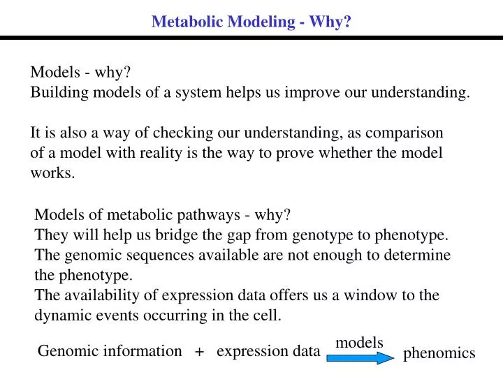
Metabolic Modeling - Why?. Models - why? Building models of a system helps us improve our understanding. It is also a way of checking our understanding, as comparison of a model with reality is the way to prove whether the model works. Models of metabolic pathways - why?

E N D
Metabolic Modeling - Why? Models - why? Building models of a system helps us improve our understanding. It is also a way of checking our understanding, as comparison of a model with reality is the way to prove whether the model works. Models of metabolic pathways - why? They will help us bridge the gap from genotype to phenotype. The genomic sequences available are not enough to determine the phenotype. The availability of expression data offers us a window to the dynamic events occurring in the cell. models Genomic information + expression data phenomics
Categorising methods (Hatzimanikatis and Bailey) Categorising models according to the interaction between a subsystem and its cellular enviroment. Isolated mechanism fixed interactions Isolated mechanism + specific growth rate one way interaction Single input-multiple output coupling specific growth rate = f (C) biochemical detail in one direction Multiple input-multiple output spectrum of interactions complexity
Categorising methods (Giuseppin and van Riel) “Engineering” approach: Input and output fluxes are measured and used to determine the internal net fluxes through the metabolic pathways. These methods are static; they describe fluxes at given conditions and do not allow for extrapolation to other conditions and transients. Example: Metabolic Flux Analysis (MFA), Flux Balance Analysis (FBA). Cybernetic approaches. Based on the hypothesis that cells react to their environment using an optimal response for survival and competition. Example: Optimal Metabolic Control Theory. Treat metabolism as a limited set of enzymes with interactions that can be described in terms of substrate, enzyme and product levels. Example: Metabolic Control Analysis.
Dynamic Optimal Metabolic Control MFA Identify the steady stases and fluxes as the OPTIMAL states under given growth rates and conditions DATA (metabolic flux info on steady states of continuous cultures of an organism) Constraints are now visible. Upper /lower limits for fluxes Identify strategies related to growth, substrate uptake and homeostasis. These form the cybernetic heart of the model. • Steady-state and dynamic modelling method. Needs data on: • relevant stoichiometric matrix • fluxes • compound concentrations
Molecular versus System Level Approaches Qualitative verbal models have been dominant in biochemistry - a young science studying unknown and complex systems. Reductionist approaches have been popular because they provided us with ever-increasing knowledge of the biochemical details of metabolic networks (pathways=>enzymes=>genes) Quantitative systems approach builds a mathematical description of the system properties based on information about general features of the molecular structure.
Metabolic Steady States Living organisms have the ability to maintain a relatively constant composition whilst taking in nutrients from the environment and excreting products. There is a constant flux of matter and energy through the metabolic pathways => dynamic equilibrium. Intermediates in the pathway must not be allowed to accumulate, so: rate of formation = rate of degradation Ethanol + CO2 1 2 3 Glucose .... Glc6P Fru6P rate 1 = rate 2 = rate 3 = ...
The quest for the rate-limiting step When a process is conditioned as to its rapidity by a number of separate factors the rate of the process is limited by the pace of the slowest factor. This statement is wrong if taken literally. In a linear metabolic pathway all reactions operate at the same rate in the steady state. What was really meant was that the rate of a pathway could be altered only by changing the activity of one particular enzyme. Despite the fact that experimental data has often contradicted this concept, much of the work on the control of metabolism has been centred around the search for potential regulatory enzymes. Regulatory enzymes were expected to: - be found at the beginning of a pathway - be non-equilibrium enzymes - show changes in activity caused not just by their own substrates - directly affect the metabolic flux
Problems with rate-limiting step approaches The rate of a sequence of simple chemical reactions could depend to varying degrees on the rate constants of all the reactions. (1930s) The rate of a sequence of unsaturated enzymes depends non-linearly on the kinetic parameters of all the enzymes. (Waley, 1964) The increase in amount of rate-limiting enzymes using gene cloning techniques did not always result in an increase of the rate of the pathway. (glycolysis experiment, 1986) Replacing the question: Is this enzyme rate-limiting? with How does this enzyme’s activity affect the metabolic flux? Use of sensitivity analysis (introduced into metabolic biochemistry by Higgins, 1960s). Biochemical Systems Theory, developed based on sensitivity analysis (Savageau, 1969). Metabolic Control Analysis (Theory) (Kacser and Burns, Heinrich and Rapoport, 1970s).
Metabolic Control Analysis - Basics En E1 Sn Z Y ... X source ... S1 product Jn J1 Flux control coefficient CE1Jn = lnJn / ln[E1] ln(Jn) For small enzyme concentration changes, the flux control coefficient can be used to calculate the flux using a power law: J = a [E]C ln([E1]) Summation theorem Kacser and Burns found that the coefficients for all enzymes that affect a particular metabolic flux in a cell, must add up to 1:
Metabolic Control Analysis - Basics (2) Elasticity e = ln|v|/ ln[S] ln(rate v) Elasticities measure the influence of metabolites on enzymes, and are thus related to the kinetic properties of the enzymes. Elasticities are properties of individual enzymes and not of the metabolic system. Elasticities can also be defined with respect to external effectors (=> response coefficients). ln([S]) The sum of the products of flux control coefficients with elasticities for all enzymes in the system is zero: Connectivity theorem
Metabolic Control Analysis - Problems • Chief intellectual achievements of MCA (Kell and Mendes, 1999): • Each step in a linear pathway at steady state contributes quantitatively to the control • of flux in a manner expressed by the summation theorem. • The flux-control coefficients are consequently necessarily small • The activities of many steps must be changed simultaneously if fluxes are to be enhanced • substantially. Implicit and explicit assumptions in MCA: All cells are the same Heterogeneity is greater than normally assumed. Simple models are adequate Many more genes than we know the functions of contribute to fitness in a cell. The “universal method” It doesn’t work if a) the end-product inhibits its proposed for large changes own synthesis and b) if there are interactions in parameters is adequate involving moiety-conserved cycles. for any metabolic system. Coefficients of MCA for very large changes are similar to those for small changes