Download
1 / 67
670 likes | 819 Views
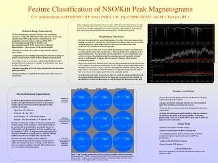
Overview of Feature Design and Classification Result. Xiang Chen Yanhua Hu Juchang Hua Ting Zhao Sept 23, 2004. 2D Cell Level Features. 2D Features Morphological Features. Contain 22 features Describing the aspect of images what human observer may pay attention to.

E N D
Overview of Feature Design and Classification Result Xiang Chen Yanhua Hu Juchang Hua Ting Zhao Sept 23, 2004
2D FeaturesMorphological Features • Contain 22 features • Describing the aspect of images what human observer may pay attention to
2D FeaturesMorphological Features Object features
Equation - COF • Center Of Fluorescence
2D FeaturesMorphological Features Object features (DNA)
(Boland and Murphy, 2001) 2D FeaturesMorphological Features # of objects Average size of objects Average distance to COF 108 83 31 6 232 4
2D FeaturesMorphological Features Edge features
Canny method of edge detection Convex Hull finding Illustration – Edge Detection and Convex Hull
2D FeaturesMorphological Features Skeleton features
Skeleton finding Illustration – Skeleton
Zernike Moment Features(SLF 3.17-3.65) • Shape similarity of protein image to Zernike polynomials Z(n,l) • 49 polynomials and 49 features left: Zernike polynomials A: Z(2,0) B: Z(4,4) C: Z(10,6) right: lamp2 image
Haralick Texture Features(SLF7.66-7.78) • Correlations of adjacent pixels in gray level images • Co-occurrence matrix P: N by N matrix, N=number of gray level. Element P(i,j) is the probability of pixels with value i being adjacent with pixels with value j • 13 statistical features
1 2 3 4 1 2 3 4 1 2 3 4 1 2 3 4 1 0 2 1 3 1 2 1 0 1 1 0 1 0 3 1 0 3 0 1 2 2 4 4 4 2 1 6 3 4 2 1 4 3 3 2 3 0 4 4 3 1 4 2 2 3 0 3 6 2 3 0 3 4 1 3 0 4 0 3 4 2 3 2 2 4 1 4 2 4 4 3 3 1 2 4 1 4 3 2 Co-occurrence Matrix
Wavelet Transformation A: approximation (low frequency) D: detail (high frequency) X=A3+D3+D2+D1
Daubechies D4 Wavelet The scaling function (for low frequency component) The mother wavelet (for high frequency component)
Daubechies D4 decompsotion Original image Wavelet Transformation
Feature Calculation • Preprocessing • Background subtraction and thresholding, • Translation and rotation • Wavelet transformation • The Daubechies 4 wavelet • 10th level decomposition • The average energy of the three high-frequency components
A 2D Gabor Function A 2D Gaussian modulated by a sinusoid
Graph for Gabor Function We can extend the function to generate Gabor filters by rotating and dilating
Feature Calculation • Preprocessing • 30 Gabor filters were generated using five different scales and six different orientations • Convolve an input image with a Gabor filter • Take the mean and standard deviation of the convolved image • 60 Gabor texture features
Different Classifiers • Decision Tree • K-NN • Neural Net • Single hidden layer • Multiple hidden layers • SVM • Linear kernel • RBF kernel • Exponential RBF kernel • Polynomial kernel • AdaBoost • Bagging • Mixture of Experts • Majority-voting Ensemble
Majority Voting Ensemble Classifier with More Features • Daubechies wavelet and Gabor transform features • SLF 15 :44 features selected by SDA from full feature set except DNA features • SLF 16: 47 features selected by SDA from full feature set including DNA features
2D FeaturesField Features • Contain 26 features • These features are not sensitive to the number of cells in the field of image • Derived from the 2D morphological features (3 obj. + 5 edge + 5 skeleton) and Haralick texture feature (13)
Field Feature ClassificationData - 10 Class mHela Images (Kai and Murphy, 2004) • Has various number (2-6) of cells • Created by randomly mixing the cropped single Hela cell images
Field Feature ClassificationMethod • SDA feature selection • 23 selected • Top 7 are Haralick texture features • Classier • DAG Gaussian-kernel SVM • Max-win multi-class strategy
Field Feature ClassificationResult (Kai and Murphy, 2004)
SLF-9 • 28 features, 14 from protein objects and 14 from their relationship to corresponding DNA images • Based on number of objects, object size, object distance to COF • Corresponding DNA image required • A subset of 9 features selected by SDA forms SLF10
SLF-14 • 14 SLF-9 features that do not require DNA images • 2 Edge features • Ratio of above threshold pixel along an edge • Ratio of fluorescence along an edge • 26 3D Haralick texture feature • GLCM built on 13 directions • One set (13) of mean features and the other set (13) of range features
Pixel Resolution and Gray Levels • Texture features are potentially influenced by the number of gray levels and pixel resolution of the image • Optimization for each image dataset required
SLF-17 • A feature subset with 7 features selected from SLF-14 at 256 gray levels and 0.4 micron pixel resolution • 1 morphological feature • 1 edge feature • 5 texture features • Achieved 98% overall accuracy in a 10-class 3D HeLa dataset
Classification using Different Feature Set • SLF-9: 91% • SLF-10: 93% • 14 morphological features from SLF-9: 86% • SLF-17: 98%
Net Benefit of 3D Texture Features • Consistently better performance using 256 gray levels compared to the other two gray levels • Comparable performance using 0.2 μm and 0.4 μm pixel resolutions
2D Object Features SOF1.1: Number of pixels in object SOF1.2: Distance between object COF and DNA COF SOF1.3: Fraction of object pixels overlapping with DNA SOF1.4: A measure of eccentricity of the object SOF1.5: Euler number of the object SOF1.6: A measure of roundness of the object SOF1.7: The length of the object’s skeleton by homotopic thinning SOF1.8: The ratio of skeleton length to the area of the convex hull of the skeleton SOF1.9:The fraction of object pixels contained within the skeleton SOF1.11: The fraction of object fluorescence contained within the skeleton SOF1.12: The ratio of the number of branch points in skeleton to length of skeleton
Feature Description • SOF1.4 A measure of eccentricity of the object • To measure the eccentricity of the ellipse that is equalivent
Feature Description • SOF1.6: A measure of roundness of the object