Download
1 / 52
830 likes | 1.58k Views
CPE 400 / 600 Computer Communication Networks. Lecture 26 Physical Layer Ch 4: Digital Transmission. Slides are modified from Behrouz A. Forouzan. Chapter 4: Digital Transmission 4.1 Digital-to-Digital Conversion Line coding Block coding Scrambling

E N D
CPE 400 / 600Computer Communication Networks Lecture 26 Physical Layer Ch 4: Digital Transmission Slides are modified from Behrouz A. Forouzan
Chapter 4: Digital Transmission 4.1 Digital-to-Digital Conversion Line coding Block coding Scrambling 4.2 Analog-to-Digital Conversion Pulse Code Modulation (PCM) Delta Modulation (DM) 4.3 Transmission Modes Parallel Transmission Serial Transmission Lecture 26: Outline
4-1 DIGITAL-TO-DIGITAL CONVERSION • We can represent digital data by using digital signals. • The conversion involves three techniques: line coding, block coding, and scrambling. • Line coding is always needed. • Block coding and scrambling may or may not be needed. Line coding and decoding
Signal element versus data element Although the actual bandwidth of a digital signal is infinite, the effective bandwidth is finite.
Example A signal is carrying data in which one data element is encoded as one signal element ( r = 1). If the bit rate is 100 kbps, what is the average value of the baud rate if c is between 0 and 1? Solution We assume that the average value of c is 1/2 . The baud rate is then
Example The maximum data rate of a channel is Nmax = 2 × B × log2 L (defined by the Nyquist formula). Does this agree with the previous formula for Nmax? Solution A signal with L levels actually can carry log2L bits per level. If each level corresponds to one signal element and we assume the average case (c = 1/2), then we have
Example In a digital transmission, the receiver clock is 0.1 percent faster than the sender clock. How many extra bits per second does the receiver receive if the data rate is 1 kbps? How many if the data rate is 1 Mbps? Solution At 1 kbps, the receiver receives 1001 bps instead of 1000 bps. At 1 Mbps, the receiver receives 1,001,000 bps instead of 1,000,000 bps.
Polar NRZ-L and NRZ-I schemes level of voltage determines value of the bit inversion or lack of inversion determines value of the bit • Both have an average signal rate of N/2 Bd. • Both have a DC component problem.
Example A system is using NRZ-I to transfer 10-Mbps data. What are the average signal rate and minimum bandwidth? Solution The average signal rate is S = N/2 = 500 kbaud. The minimum bandwidth for this average baud rate is Bmin = S = 500 kHz.
Polar biphase: Manchester and differential Manchester schemes • Transition at the middle is used for synchronization • The minimum bandwidth is 2 times that of NRZ
Bipolar schemes: AMI and pseudoternary We use three levels: positive, zero, and negative. • In mBnL schemes, a pattern of m data elements is encoded as a pattern of n signal elements in which 2m ≤ Ln
Block coding concept Block coding is normally referred to as mB/nB coding; it replaces each m-bit group with an n-bit group.
Example We need to send data at a 1-Mbps rate. What is the minimum required bandwidth, using a combination of 4B/5B and NRZ-I or Manchester coding? Solution First 4B/5B block coding increases the bit rate to 1.25 Mbps. The minimum bandwidth using NRZ-I is N/2 or 625 kHz. The Manchester scheme needs a minimum bandwidth of 1 MHz. The first choice needs a lower bandwidth, but has a DC component problem; The second choice needs a higher bandwidth, but does not have a DC component problem.
Two cases of B8ZS scrambling technique B8ZS substitutes eight consecutive zeros with 000VB0VB.
Different situations in HDB3 scrambling technique HDB3 substitutes four consecutive zeros with 000V or B00V depending on the number of nonzero pulses after the last substitution.
Chapter 4: Digital Transmission 4.1 Digital-to-Digital Conversion Line coding Block coding Scrambling 4.2 Analog-to-Digital Conversion Pulse Code Modulation (PCM) Delta Modulation (DM) 4.3 Transmission Modes Parallel Transmission Serial Transmission Lecture 26: Outline
4-2 ANALOG-TO-DIGITAL CONVERSION • A digital signal is superior to an analog signal. • The tendency today is to change an analog signal to digital data. • In this section we describe two techniques, pulse code modulation and delta modulation.
Nyquist sampling rate for low-pass and bandpass signals According to the Nyquist theorem, the sampling rate must be at least 2 times the highest frequency contained in the signal.
Recovery of a sampled sine wave for different sampling rates Sampling at the Nyquist rate can create a good approximation of the original sine wave. Oversampling can also create the same approximation, but is redundant and unnecessary. Sampling below the Nyquist rate does not produce a signal that looks like the original sine wave.
Sampling of a clock with only one hand The second hand of a clock has a period of 60 s. According to the Nyquist theorem, we need to sample hand every 30 s
Examples An example of under-sampling is the seemingly backward rotation of the wheels of a forward-moving car in a movie. A movie is filmed at 24 frames per second. If a wheel is rotating more than 12 times per second, the under-sampling creates the impression of a backward rotation. Telephone companies digitize voice by assuming a maximum frequency of 4000 Hz. The sampling rate therefore is 8000 samples per second.
Example A complex low-pass signal has a bandwidth of 200 kHz. What is the minimum sampling rate for this signal? Solution The bandwidth of a low-pass signal is between 0 and f, where f is the maximum frequency in the signal. Therefore, we can sample this signal at 2 times the highest frequency (200 kHz). The sampling rate is therefore 400,000 samples per second.
Example A telephone subscriber line must have an SNRdB above 40. What is the minimum number of bits per sample? Solution We can calculate the number of bits as Telephone companies usually assign 7 or 8 bits per sample.
Example We want to digitize the human voice. What is the bit rate, assuming 8 bits per sample? Solution The human voice normally contains frequencies from 0 to 4000 Hz. So the sampling rate and bit rate are calculated as follows:
Example We have a low-pass analog signal of 4 kHz. If we send the analog signal, we need a channel with a minimum bandwidth of 4 kHz. If we digitize the signal and send 8 bits per sample, we need a channel with a minimum bandwidth of 8 × 4 kHz = 32 kHz.
Chapter 4: Digital Transmission 4.1 Digital-to-Digital Conversion Line coding Block coding Scrambling 4.2 Analog-to-Digital Conversion Pulse Code Modulation (PCM) Delta Modulation (DM) 4.3 Transmission Modes Parallel Transmission Serial Transmission Lecture 26: Outline
4-3 TRANSMISSION MODES • The transmission of binary data across a link can be accomplished in either parallel or serial mode. • In parallel mode, multiple bits are sent with each clock tick. • In serial mode, 1 bit is sent with each clock tick. • While there is only one way to send parallel data, there are three subclasses of serial transmission: asynchronous, synchronous, and isochronous.