Download
1 / 12
120 likes | 212 Views
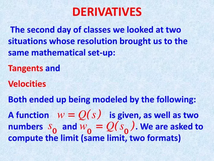
DERIVATIVES. The second day of classes we looked at two situations whose resolution brought us to the same mathematical set-up: Tangents and Velocities Both ended up being modeled by the following:

E N D
DERIVATIVES The second day of classes we looked at two situations whose resolution brought us to the same mathematical set-up: Tangents and Velocities Both ended up being modeled by the following: A function is given, as well as two numbers and . We are asked to compute the limit (same limit, two formats)
or In fact, computing these limits is one of the reasons we studied limits in the first place. The ratios are called difference quotient. Let us interpret all of this for tangents and for velocities.
Let’s start by observing that writing out a difference ratio is rather cumbersome! We need a slicker notation. If you note that the difference quotient for a function looks like, in either one of the two versions, as , we see that all we need is
a slick notation for “change in anything”. Mathematicians invented such a notation a few years back, it is written as so that for the function the difference quotient is written as And for the more familiar function we get .
Let’s look at a picture. If the function shown is just a nice curve the difference quotient is just rise/run = the slope of the secant. In the limit we get
the slope of the tangent. If the function shown expresses a quantity that changes as time changes, the difference quotient is the average rate of change over the time interval In the limit we get the instantaneous rate of change.
When the quantity represents distance traveled in time we call the instantaneous rate of change the instantaneous velocity at time All of these examples reduce to having to compute the limit of a difference quotient when the “bottom” approaches 0. So, first of all, …. we formalize this procedure with the following
Definition. Let be defined near and at the point . The derivative of at is if the limit exists. Notation. When the limit exists we denote its value (that clearly depends on and ) by (also by and by or anything else that indicates you computed the above limit using and .
Computing derivatives from scratch is no picnic, we will look for ‘laws’ (as we did for limits !) to make our life easier. In the meantime, to keep ourselves honest, let’s do some computations of derivatives (tangents or velocities, I’ll change the question, but the answers will still be computing the limits of difference quotients !) Problem 1. Find the equation of the tangent to at the point .
First of all, what’s the value of ? Any takers? That’s right, it is ….. . Here is an (approximate) graph To get the slope of the tangent we must find
the limit that is A little 7th grade algebra shows that
reduces to: So the slope of the tangent is 4 and we can find its equation, since we know it goes through , We get