Acceleration analysis (Chapter 4)

1. Acceleration analysis (Chapter 4) • Objective: Compute accelerations (linear and angular) of all components of a mechanism

2. Outline • Definition of acceleration (4.1, 4.2) • Acceleration analysis using relative acceleration equations for points on same link (4.3) • Acceleration on points on same link • Graphical acceleration analysis • Algebraic acceleration analysis • General approach for acceleration analysis (4.5) • Coriolis acceleration • Application • Rolling acceleration

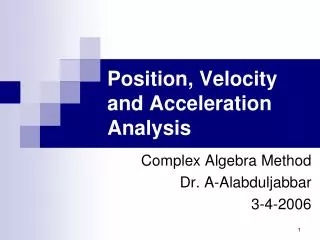
3. Definition of acceleration (4.1, 4.2) • Angular = = rate of change in angular velocity • Linear = A = rate of change in linear velocity (Note: a vector will be denoted by either a bold character or using an arrow above the character)

4. Acceleration of link in pure rotation (4.3) AtPA P APA Length of link: p AnPA ,   A Magnitude of tangential component = p, magnitude of normal component = p 2

5. Acceleration of link, general case AtPA P APA Length of link: p AnPA ,   AnPA AtPA AP A APA AA AA AP=AA+APA

6. Graphical acceleration analysis Four-bar linkage example (example 4.1) AtBA B AtB 3 A AtA 4 Clockwise acceleration of crank 2 AnA 1

7. Problem definition: given the positions of the links, their angular velocities and the acceleration of the input link (link 2), find the linear accelerations of A and B and the angular accelerations of links 2 and 3. Solution: • Find velocity of A • Solve graphically equation: • Find the angular accelerations of links 3 and 4

8. B AtB 3 A 2 AtA 4 AnA 1 Graphical solution of equationAB=AA+ABA AtB AtBA AA AtBA AnBA -AnB • Steps: • Draw AA, AnBA, -AtBA • Draw line normal to link 3 starting from • tip of –AnB • Draw line normal to link 4 starting from origin of AA • Find intersection and draw AtB and AtBA.

9. Guidelines • Start from the link for which you have most information • Find the accelerations of its points • Continue with the next link, formulate and solve equation: acceleration of one end = acceleration of other end + acceleration difference • We always know the normal components of the acceleration of a point if we know the angular velocity of the link on which it lies • We always know the direction of the tangential components of the acceleration

10. 3 B A b c 2 4 a 1 Algebraic acceleration analysis (4.10) R3 R4 R2 R1 1 Given: dimensions, positions, and velocities of links and angular acceleration of crank, find angular accelerations of coupler and rocker and linear accelerations of nodes A and B

11. Loop equation Differentiate twice: This equation means:

12. Solution

13. General approach for acceleration analysis (4.5) • Acceleration of P = Acceleration of P’ + Acceleration of P seen from observer moving with rod+Coriolis acceleration of P’ P, P’ (colocated points at some instant), P on slider, P’ on bar

14. Coriolis acceleration Whenever a point is moving on a path and the path is rotating, there is an extra component of the acceleration due to coupling between the motion of the point on the path and the rotation of the path. This component is called Coriolis acceleration.

15. Coriolis acceleration APslip: acceleration of P as seen by observer moving with rod VPslip P APcoriolis AP’n AP’t APslip O AP

16. Coriolis acceleration • Coriolis acceleration=2Vslip • Coriolis acceleration is normalto the radius, OP, and it points towards the left of an observer moving with the slider if rotation is counterclockise. If the rotation is clockwise it points to the right. • To find the acceleration of a point, P, moving on a rotating path: Consider a point, P’, that is fixed on the path and coincides with P at a particular instant. Find the acceleration of P’, and add the slip acceleration of P and the Coriolis acceleration of P. • AP=acceleration of P’+acceleration of P seen from observer moving with rod+Coriolis acceleration=AP’+APslip+APCoriolis

17. Application: crank-slider mechanism B2 on link 2 B3 on link 3 These points coincide at the instant when the mechanism is shown. When 2=0, a=d-b Unknown quantities marked in blue . B2, B3 normal to crank Link 2, a 3, 3, 3 2, 2 2 O2 Link 3, b d

18. General approach for kinematic analysis • Represent links with vectors. Use complex numbers. Write loop equation. • Solve equation for position analysis • Differentiate loop equation once and solve it for velocity analysis • Differentiate loop equation again and solve it for acceleration analysis

19. Position analysis Make sure you consider the correct quadrant for 3

20. Velocity analysis VB3= VB2+ VB3B2 VB3B2 // crank VB3┴ rocker B2 on crank, B3, on slider . crank VB2 ┴ crank rocker O2

21. Velocity analysis is the relative velocity of B3 w.r.t. B2

22. Acceleration analysis Where:

23. Relation between accelerations of B2 (on crank) and B3 (on slider) AB3slip // crank AB3 Crank . B2, B3 AB3Coriolis ┴ crank AB2 Rocker

24. Rolling acceleration (4.7) First assume that angular acceleration, , is zero O  O   (absolute) R C  (absolute) C r P No slip condition: VP=0

25. Find accelerations of C and P • -(R-r)/r (Negative sign means that CCW rotation around center of big circle, O, results in CW rotation of disk around its own center) • VC= (R-r) (Normal to radius OC) • AnC=VC2/(R-r) (directed toward the center O) • AnP=VC2/(R-r)+ VC2 /r (also directed toward the center O) • Tangential components of acceleration of C and P are zero

26. Summary of results AC, length VC2/(R-r) R C VC, length (R-r) r AP, length VC2/(R-r)+ VC2 /r P VP=0

27. Inverse curvature •  (R+r)/r • VC=(R+r) (normal to OC) • AnC=VC2/(R+r) (directed toward the center O) • AnP=VC2/r - VC2 /(R+r) (directed away from the center O) • Tangential components of acceleration are zero

28. Inverse curvature: Summary of results VC, length (R+r) C r AC, length VC2/(R+r) P VP=0 R AP, length VC2 /r -VC2/(R+r)

29. Now consider nonzero angular acceleration, 0 • The results for zero angular acceleration are still correct, but • ACt=r (normal to OC) • APt is still zero • These results are valid for both types of curvature