Download
1 / 65
650 likes | 745 Views
Intermediate Statistical Analysis Professor K. Leppel. Hypothesis Testing. One Sample. Notation. H 0 : hypothesis being tested “null hypothesis” H a or H 1 : alternative hypothesis. Example: H 0 : = 100 versus H 1 : 100.

E N D
Hypothesis Testing One Sample
Notation H0: hypothesis being tested “null hypothesis” Ha or H1: alternative hypothesis Example: H0: = 100 versus H1: 100
Type I and Type II errors • Type I error – rejecting the null hypothesis when it’s true. • Type II error – accepting the null hypothesis when it’s false.
Critical region • Values of the test statistic for which the null hypothesis is rejected. • Example: Suppose you are testing whether or not the population mean is 100. • Your test statistic is the sample mean. • If the sample mean is very far from 100, perhaps less than 90 or more than 110, you reject the hypothesis that the mean is 100. • Then your critical region is the set of values of the sample mean that are less than 90 or more than 110.
Acceptance region • Values of the test statistic for which the null hypothesis is accepted. • Example: Again suppose you are testing whether the population mean is 100, and your test statistic is the sample mean. • You decided to reject the null hypothesis if the sample mean is less than 90 or more than 110. • You accept the null hypothesis if the sample mean is between 90 and 110. • Then your acceptance region is the set of values of the sample mean that are between 90 and 110.
Example: Suppose you want to know whether the mean IQ at a particular university is 130. You know the population standard deviation is 5.4. To test the hypothesis, you take a random sample of 25 observations. The mean IQ of the sample is 128.
If the null hypothesis is correct, the center of the distribution of the sample mean is 130. Our critical and acceptance regions look like this graph. We need to determine what a and b are so that we know when we should accept our null hypothesis and when we should reject it. acceptance region crit. reg. crit. reg. a 130 b
Suppose we want our probability of type I error to be at most 0.05. We want the probability of rejecting the null hypothesis when it is actually correct to be 0.05. So we are in the critical region when the graph is centered at 130 with probability 0.05. The area in each of the two tails of the critical region is half of 0.05 or 0.025. acceptance region 0.025 0.025 crit. reg. crit. reg. a 130 b
The equation we derived implies this graph of the standard normal or Z distribution. From the Z table, we know that the cut-off points for the tails with area 0.025 must be 1.96 and -1.96. -1.96 1.96 .025 .025
Solving the first equation for a and the second equation for b, we find a = 127.88 and b = 132.12.
Returning to our graph for the sample mean, we have this picture. So if our sample mean is between 127.88 and 132.12, we accept the null hypothesis that the population mean IQ is 130. If our sample mean is less than 127.88 or more than 132.12, we reject the null hypothesis and accept the alternative that the population mean is not 130. acceptance region crit. reg. crit. reg. 127.88 130 132.12
Since the sample mean was 128, what would our decision be? Accept H0: = 130 If the sample mean was 127 instead, what would our decision be? acceptance region crit. reg. crit. reg. 127.88 130 132.12
In the hypothesis test we just performed, we determined the cut-off points a and b for the sample mean, and then checked to see if our observed values were in the acceptance or critical region. • Another way of doing the hypothesis test is to use the “p-value.” • The p-value is the probability that the value of the sample mean is as far away from the hypothesized mean as observed, if the hypothesized mean is actually correct. • If the p-value is greater than our test level , we accept the null hypothesis. • If the p-value is less than , we reject the null hypothesis. • The reasoning when the p-value is less than is this: • The probability of seeing the observed value of the sample mean, if the null hypothesis is true, is very small. Since it’s unlikely under the assumption of the null hypothesis, we reject that hypothesis.
Let’s do the same problem using the p-value method. Recall that the sample mean was 128, the population standard deviation was 5.4, the sample size was 25, and the test level was 0.05. .4678 .4678 .0322 .0322 -1.85 0 1.85 Z = 2 (0.5-0.4678) = 2 (0.0322) = 0.0644 Using a test level of = 0.05, we accept the null hypothesis, since the p-value > 0.05 .
Quick & Dirty Method of Hypothesis Testing • Convert the sample mean to a standard normal Z-statistic: 2. Sketch the critical & acceptance regions in terms of a Z-statistic. 3. Make the decision.
Same problem one more time: Recall that the sample mean was 128, the population standard deviation was 5.4, the sample size was 25, and the test level was 0.05. crit. reg. crit. reg. .4750 .4750 .0250 .0250 -1.96 0 1.96 Z Based on a test level or of 0.05, we have the graph below. Since the Z-value -1.85 is in the acceptance region, we accept the null hypothesis that the population mean is 130.
When a hypothesis has only one value such as = 130, we call it a simple hypothesis. When a hypothesis has more than one value, we call it a composite hypothesis. Some examples:
The critical region depends on the alternative hypothesis, not the null. If the alternative is “not equal to”, the critical region is 2-tailed. If the alternative is “greater than”, the critical region is the right tail only. If the alternative is “less than”, the critical region is the left tail only.
1-Tailed Hypothesis Test at the 5% level if the sample mean is 128 based on a sample of size 25, and the population standard deviation is 5.4. • We will again use these 3 methods to do this problem: • Determine critical region in terms of the sample mean. • P-value • “Quick & Dirty”
1. Determine critical region in terms of the sample mean. We sketch the graph under the assumption that the null hypothesis is true, centering the graph at the most conservative value of that hypothesis, = 130. .45 crit. reg. Acceptance region .05 130 a Since the alternative hypothesis is <130, the critical region is the left tail. Since the test level is 5%, the area of the critical region is 0.05.
crit. reg. .45 Acceptance region .05 0 Z crit. reg. .45 Acceptance region .05 130 a Using the Z table, we find the cut-off point must be -1.645.
.45 crit. reg. Acceptance region .05 a 130 128.22 we find a = 128.22. Our value of the sample mean was 128. Since 128 is in the critical region, we reject the null hypothesis and accept the alternative that < 130.
2. P-value method. Keep in mind that the sample mean is 128, the population standard deviation is 5.4, the sample size is 25, and the test level is 0.05. .0322 0 -1.85 Z Using a test level of = 0.05, we reject the null hypothesis and accept the alternative that <130, since the p-value < 0.05 . = 0.5 – 0.4678 = 0.0322
3. “Quick & Dirty” Method. Again, remember that the sample mean was 128, the population standard deviation was 5.4, the sample size was 25, and the test level was 0.05. Based on a test level or of 0.05, we have the graph below. crit. reg. .45 Acceptance region .05 0 -1.645 Z Since the Z-value -1.85 is in the critical region, we reject the null hypothesis and accept the alternative that < 130.
Calculating Recall that is the probability of type I error = Pr( reject H0 | H0 is true), and is the probability of type II error = Pr( accept H0 | H0 is false).
where the population standard deviation is 50 and the sample size is 25. Let’s first determine the critical region, and then calculate , based on a specified value of .
acceptance region 0.025 0.025 crit. reg. crit. reg. a 1000 b
The above equation implies this graph of the standard normal or Z distribution. From the Z table, we know that the cut-off points for the tails with area 0.025 must be 1.96 and -1.96 -1.96 1.96 .025 .025
acceptance region crit. reg. crit. reg. 980.4 1000 1019.6 Solving the first equation for a and the second equation for b, we find a = 980.4 and b = 1019.6. So our critical and acceptance regions look like this:
But what if is actually 990, not 1000? acceptance region crit. reg. crit. reg. 980.4 990 1019.6 Our cut-off values for the critical and acceptance regions are still the same, but the distribution curve is centered at 990 instead of at 1000. = Pr(accepting H0| H0 is false, in this case, =990) = Pr(being in acceptance region| =990)
.3315 .4985 -0.96 0 2.96 Z We determine from the Z table that the specified area is 0.3315 + 0.4985 = 0.83
So, , the probability of accepting the null hypothesis that = 1000, when is actually 990, is 0.83. • With the given standard deviation and sample size, it is difficult to distinguish a distribution with a mean of 990 from a distribution with a mean of 1000. • If we had a mean of 900, which is farther from 1000 than 990 is, it would be easier to distinguish it from 1000, and our value of would be smaller.
In general, we want the probability of type I and type II errors, and , to be small. How can we make and smaller? Since is the probability of accepting the null hypothesis when it is false, we can make smaller by accepting the null hypothesis less often (shrinking the acceptance region). If we shrink the acceptance region, however, we expand the critical region. That means we reject the null hypothesis more often, increasing the probability of rejecting it when it is correct. So we’ve increased . Similarly, if we try to decrease , we increase .
Example: Parties Suppose you have just completed your first semester at college. You are reflecting back on your social experiences of the semester, and thinking that you went to a lot of boring parties. You are thinking that you would like to reduce the number of boring parties that you attend. Think of the decision to attend a party as one involving the null hypothesis that the party is a good one and the alternative hypothesis is that the party is boring. You want to keep down the error probabilities = Pr(skip a party | it’s a good one) and = Pr(attend a party | it’s boring). To reduce , you might go to a lot of parties, but then you risk attending boring ones. To reduce , you might go to very few parties, but then you risk missing some good ones.
Is there some way that we can decrease both and ? • Yes, we can decrease both and by collecting more data or more information, by increasing the sample size. • Unfortunately, in the real world, collecting more data usually means increasing the cost of the study. • So there’s a tradeoff between accuracy and cost.
In the context of our party example, to keep down the number of boring parties you attend as well as the number of good parties you miss, you need to get more information. You need to talk to more people, find out who’s going, the music that is likely to be played, the food that will be served, etc.
How do we do hypothesis testing when the population standard deviation is unknown? We do it similarly to what we’ve done so far, but we replace the population standard deviation by the sample standard deviation and the Z distribution by the t distribution
Example: Suppose you sample 16 matchboxes. The sample mean number of matches per box is 17 and the sample standard deviation is 2. Test at the 5% level Use all three methods that we used previously.
Method 1 If the null hypothesis is correct, the distribution of the sample mean is centered at 18. We need to find the values of a and b so that the combined area in the two tails is 0.05. We don’t have to compute a and b separately. We can just compute one of them and figure out the other by symmetry. We’ll do b. acceptance region 0.025 0.025 crit. reg. crit. reg. a 18 b
The equation we derived implies this graph of the t distribution. From the t table, we find that for 15 degrees of freedom, the cut-off points for the two tails with a combined area 0.05 are 2.131 and -2.131. -2.131 2.131 .025 .025
Solving the first equation for a and the second equation for b, we find a = 16.93 and b = 19.07, which gives us the acceptance and critical regions shown in the graph. Since our value for the sample mean is 17, which is in the acceptance region, we accept the null hypothesis that = 18. acceptance region crit. reg. crit. reg. 16.93 19.07 18