Download
1 / 25
460 likes | 1.28k Views
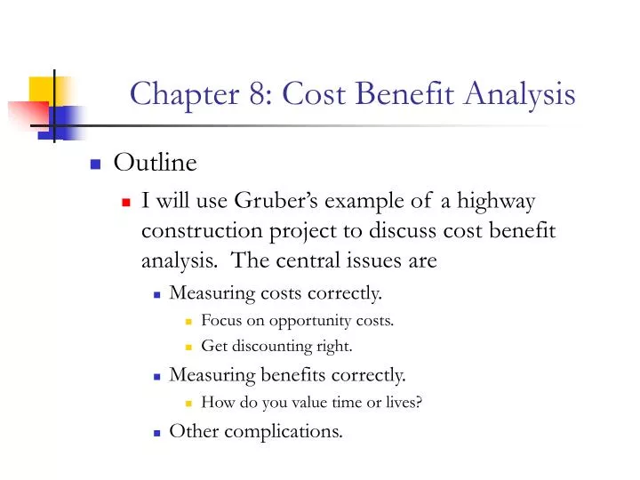
Chapter 8: Cost Benefit Analysis . Outline I will use Gruber’s example of a highway construction project to discuss cost benefit analysis. The central issues are Measuring costs correctly. Focus on opportunity costs. Get discounting right. Measuring benefits correctly.

E N D
Chapter 8: Cost Benefit Analysis • Outline • I will use Gruber’s example of a highway construction project to discuss cost benefit analysis. The central issues are • Measuring costs correctly. • Focus on opportunity costs. • Get discounting right. • Measuring benefits correctly. • How do you value time or lives? • Other complications.
Chapter 8: Cost Benefit Analysis • The government often uses cost-benefit analysis to compare the costs and benefits of public goods projects and to decide if they should be undertaken. • In principle, cost benefit analysis seems like an accounting exercise. • In practice, cost-benefit analyses are rich economic exercises that combine theory and empirical work. • The required reading for today gives an excellent overview on “real world” cost benefit analysis.
MEASURING THE COSTS OF PUBLIC PROJECTS: The Example • Consider the example of renovating a turnpike that is in poor shape, with large potholes and crumbling shoulders that slow down traffic and pose an accident risk. • Should the government repair the road? • Valuing the costs • Asphalt, labor, maintenance, and • Benefits • Driving time speed and lives saved
Table 1 The project requires several inputs – materials, labor, and maintenance over time. And it produces two main benefits – reduced commuting time and fewer fatalities.
Measuring Costs (Current and Future) • The first goal is to measure current costs. The cash-flow accounting approach to costs simply adds up what the government pays for all the inputs. • This does not represent the social marginal cost we used in the theoretical public goods analysis, however. • The social marginal cost of any resource is its opportunity cost–the value of that input in its next best use. • This is not necessarily its cash costs. Instead, you must think about what else society could do with the input.
Measuring Current (and Future) Costs • The asphalt is easy. • The next best use is to sell the bag to someone else. The value of the alternative use is given by the market price. • If the labor market is perfectly competitive, the same logic applies for labor costs. • The value of an hour of labor used on the project is simply the market wage. • If there are imperfect markets, however, then there could be unemployment. • Imagine that those who were involuntarily unemployed had a reservation wage of $5/hour; thus, they value their leisure at $5/hour.
Measuring Current Costs • In this case, the “alternative activity” is not working at another job, but rather being unemployed. • This alternative activity only has an opportunity cost of $5/hour, not $20/hour. • This lowers the economic costs of the project (but not the accounting costs). • The unemployed workers derive rents, if they are hired for the project. • Rents are simply payments to resource deliverers that exceed those necessary to employ the resource.
Table 2 For asphalt, the next best use besides using it on a project is to sell it to someone else. The value is then the market price of $100. If the labor market were competitive, the market wage rate for construction workers would completely determine the price. On the other hand, if there is involuntary unemployment. The opportunity cost for these workers is lower than the wage rate ($5). For these formerly unemployed workers, paying $20 an hour consists of a $5 opportunity cost and a $15 transfer. The accounting cost equals $20/hour x 1 million hours, or $20 million. The economic cost equals $20/hour x 0.5 million hours plus $5/hour x 0.5 million hours, for a total of $12.5 million.
Measuring Future Costs • The present discounted value of maintenance costs is computed as: • How do we convert this infinite sum into something manageable? Multiply by (1+r): • Subtract the first from the second, and get r(PDV)=C, or PDV=C/r
Measuring Future Costs • The asphalt and labor costs are immediate costs, but the last one–construction–is a stream of costs over time. • This cost is $10 million per year into the indefinite future. From the previous slide, we know this cost is C/r. But what r should we use? • Choosing the right social discount rate. • For a private firm, the answer would be the opportunity cost of what else the firm could do with the same funds, that is, the after tax rate of return. • The government should base its discount rate on the private sector opportunity cost, but the government counts both the after-tax portion of the return and the taxes collected. • An OMB directive in 1992 said the government should use 7% for all public investment projects, which is the historical pre-tax rate of return on private investments.
Table 3 The OMB suggests a 7% discount rate. Which leads to a present discounted value of $143 million (=$10 million/7%). The first year cost of the project is $112.5 million. The total cost of the project is $255.5 million.
THE BENEFITS: Valuing Driving Time Saved • For consumers, we need some measure of society’s valuation of time. There are several approaches to measuring this: • Market based measures: Wages • Survey based measures: Contingent valuation • Revealedpreference measures
The Benefits: Valuing Driving Time Saved • Use the market: • For producers, the decreased costs shift the supply curve to the right (outward), leading to an increase in the total surplus. Assuming we have estimates of supply and demand in the output market, this is straightforward. • For consumers: if we had a perfectly functioning labor market, we could “cash out” the value of the time savings, a market-based measure. • Assuming the person can freely choose the hours he wants to work, then even if the time is spent on leisure, the appropriate valuation of the time is the wage rate. • The market based approach runs into problems if hours of work are “lumpy” or if there are important non-monetary aspects of the job.
The Benefits: Valuing Driving Time Saved • Contingent valuation is a method of asking individuals to value an option they are not now choosing. • In some circumstances, this is the only feasible method for valuing a public good. • For example, there is no obvious market price to use to value saving a rare species of owl. But there are obviously huge problems with this approach. • It is very hard to design a survey that elicits true willingness to pay. • People can say most anything in a survey that has no real consequences for their lives.
The Benefits: Valuing Driving Time Saved • Another approach to valuing time is to use revealed preference–let the actions of individuals reveal their valuation. • For example, if one compared house prices for two houses, one of which was 5 minutes closer to the workplace, this would effectively “cash out” the value of saved commuting time. • In practice, this approach runs into problems because the two homes are not identical. • Some of the differences (e.g., housing attributes) can be observed and accounted for with cross sectional regression. Decomposing a sale price by its attributes is the basis of hedonic market analysis. • Other differences are either hard to measure or unobserved, however, which leads to bias.
Valuing time savings • One clever quasi-experiment to reveal the value of saved time was conducted by Deacon and Sonstelie (1985): • During the oil crisis of the 1970s, the government imposed price ceilings on gasoline of large gasoline stations, but not independent ones. • As a consequence, long lines formed at these cheaper, corporate gasoline stations. • At Chevron stations in California, gasoline was approximately 39.5¢ lower, with an average wait time of roughly 14.6 minutes. The mean purchase was around 10.5 gallons. • Thus, the tradeoff is waiting 14.6 minutes to save about $4.15, or one hour for $17. This corresponded very closely to the average hourly wage in the U.S.
The Benefits: Valuing Saved Lives • The other main benefit of the turnpike improvement is valuing saved lives due to lower traffic fatalities. • Valuing life runs into ethical issues, but almost all economists would agree that it is necessary for public policy decisions. • By stating that life is priceless or should not be valued, we leave ourselves helpless when facing choices of different programs that could each save lives. • As with valuing time savings, there are three main approaches to valuing saved lives: • Using wages • Contingent valuation • Revealed preference
The Benefits: Valuing Saved Lives • The market-based approach uses wages; the value of the life is the present discounted value of the lifetime stream of earnings. • One key problem is that this approach does not value leisure. • One set of estimates is that the average 20 year old women’s life is $3.1 million. Men are slightly higher (because of higher earnings). Old people are lower, since they have fewer years to live. • The contingent valuation approach asks people what their lives are worth. • There is obvious difficulty in a question like this, so it is often framed in terms of changes in the probability of dying. • For example, how much more would you pay for an airline ticket with a 1 in 500,000 chance of a crash compared with a 2 in 500,000 chance? • The estimates from contingent valuation have a very wide range, going from $825,000 to $22.3 million per life saved.
The Benefits: Valuing Saved Lives • The revealed preference approach examines how much individuals are willing to pay for something that reduces their odds of dying. • For example, suppose a consumer purchases an airbag for $350 that has a 1 in 10,000 chance of saving her life. The implicit valuation on life is $3.5 million. • Or examine risky jobs: • Suppose that one job has a 0.5% higher risk of death but pays $15,000 more in salary. • The $15,000 extra salary is known as the compensating differential. • The implicit valuation of life in this example is $3 million ($15,000/0.005).
Valuing Saved Lives • There is a large literature in economics using these revealed preference approaches. Viscusi estimates that the value of life is roughly $7 million. • There are drawbacks, however. • Strong information assumptions about probabilities. • Assumes people are well prepared to evaluate these tradeoffs. • Difficult to control for other attributes of the job. • Differences in valuation of life (e.g., degree of risk aversion).
Table 5 Assume we can value the driving time saved to both producers and consumers at $17 per hour. The resulting time savings per year is $8.5 million. Also, assume that the value of a life saved is $7 million. The resulting value of life savings is $35 million per year. The first year benefits are therefore $43.5 million. Applying the 7% discount rate, the total benefit is $621 million ($43.5/0.07). The benefits of the turnpike project considerably exceed the costs.
PUTTING IT ALL TOGETHER • Since the benefits exceed the costs, we would recommend the government pursue the project. • The government needs to consider one additional factor beyond the benefits and costs of the project itself: the budgetary cost of raising the funds to finance the project. • Economists typically assume some efficiency cost, or deadweight loss, from raising the tax burden to finance this spending. If the efficiency cost of raising the money is too high, some projects will not survive the cost-benefit analysis.
Other Issues: Discounting Future Benefits • A particularly thorny issue for cost-benefit analysis is that the costs are mostly short-term, while the benefits are mostly long term. • Global warming is a good example. • This may be problematic because: • The choice of discount rate will matter enormously for benefits that are far in the future. • The benefits are spread out over current and future generations.
Other Issues in Cost-Benefit Analysis • Common counting mistakes include: • Counting secondary benefits (like commerce that is simply shifted from one area to another). • Counting labor (reducing unemployment, for example) as a benefit rather than a cost. • Double counting benefits (like the value of an irrigation project to farm income, and simultaneously the increase in the value of the land).
Other Issues in Cost-Benefit Analysis • There are also distributional concerns: • The costs and benefits of a public project do not necessarily accrue to the same individuals. • In principle, a project that improved social welfare could then involve redistribution, but in practice this rarely happens. • So one might be concerned if all the benefits accrue to one group and all the costs are borne by another, particularly if the group that benefits is affluent and the group bearing the costs is poor.