Download
1 / 55
780 likes | 1.28k Views
Chapter 5: Optical Amplifiers. 5.1 Basic Concepts 5.1.1. Introduction 5.1.2. Gain Spectrum and Bandwidth 5.1.3. Gain Saturation 5.1.4. Amplifier Noise 5.1.5. Amplifier Applications 5.2 Semiconductor Optical Amplifiers 5.2.1. Amplifier Design

E N D
Chapter 5: Optical Amplifiers 5.1 Basic Concepts 5.1.1. Introduction 5.1.2. Gain Spectrum and Bandwidth 5.1.3. Gain Saturation 5.1.4. Amplifier Noise 5.1.5. Amplifier Applications 5.2 Semiconductor Optical Amplifiers 5.2.1. Amplifier Design 5.2.2. Amplifiers Characteristics 5.2.3. Pulse Amplification 5.2.4. System Application 5.3 Raman Amplifier 5.3.1. Introduction 5.3.2. Raman Gain and Bandwidth 5.3.3. Amplifier Characteristics 5.3.4. Raman Amplifier Performance
Chapter 5: Optical Amplifiers 5.4 Erbium-Doped Fiber Amplifiers 5.4.1. Introduction 5.4.2. Pumping Requirement 5.4.3. Gain Spectrum 5.4.4. Simple Theory of EDFAs 5.4.5. Amplifier Noise 5.4.6. Multi-channel Amplification 5.4.7. Distributed-Gain Amplifiers 5.5 System Applications 5.5.1. Optical Pre-amplification 5.5.2. Noise Accumulation in Long-Haul System 5.5.3. ASE-Induced Timing Jitter 5.5.4. Accumulated Dispersive and Nonlinear Effects 5.5.5. WDM-Related Impairments
5.1: Basic Concepts 5.1.1. Introduction • Electric regenerators become quite complex and expensive for WDM lightwave systems. • A homogeneously broadening two-level system with gain coefficient g(w) = go/[1+(w-wo)2T22 + P/Ps] where go is the peak value of the gain w is the optical frequency wo is the atomic transition frequency P is the signal power T2 is the dipole relaxation time < 1ps Ps is the saturation power dependent on T1 and cross section T1 is the population relaxation time: 100ps ~ 1ms.
5.1: Basic Concepts 5.1.2. Gain Spectrum and Bandwidth • The unsaturated region, P/Ps << 1, the gain spectrum g(w) and the gain bandwidth Dng (FWHM) are g(w) = go/[1+(w-wo)2T22] Dng = Dwg/2p = 1/(pT2) ~ 5 THz for SOA. • The amplifier bandwidth at FWHM of G(w,z) DnA = Dng.[ln2/ln(Go/2)]1/2 < Dng where G(w,z) = Pout/Pin = exp[g(w)z] Go = exp(goL)
5.1: Basic Concepts 5.1.3. Gain Saturation • For large signal, dP(z)/dz = goP/(1+P/Ps) with b.c. P(0) = Pin, P(L) = Pout = GPin • Thelarge-signal amplifier gain G = P/Pin= Goexp[-(G-1)Pout/GPs] • The output saturation power: the output power for which G = Go/2 Psout = PsGoln2/(Go-2) ~ 0.69Ps for Go > 20dB
5.1: Basic Concepts 5.1.4. Amplifier Noise • Resulted from the beating of spontaneous emission with the signal. • Amplifier noise figure Fn = (SNR)in/(SNR)out • The SNR of the input signal (SNR)in = <I>2/ss2 = (RPin)2/2q(RPin)Df = Pin/2hnDf where <I>is the average photocurrent • ss2 is the shot noise by setting the dark current zero, and Df is the detector bandwidth.
5.1.4. Amplifier Noise • The spectral density of spontaneous-emission-induced noise Ssp(n) = (G-1)nsphn is nearly constant • The spontaneous-emission factor (the population inversion factor) nsp= N2/(N2-N1), N1, N2 being populations for the ground and the excited states. • The mixed photocurrent I = R |√G Ein + Esp|2 • The beat noise current and its variance DI = 2R(GPin)1/2|Esp|2 , s2 ~ 4(RGPin)(RSsp)Df • The SNR of the amplified signal (SNR)out = <I>2/s2 ~ GPin/4SspDf • Noise figure : Fn=2nsp(G-1)/G ~ 2nsp ~ 5.8 dB
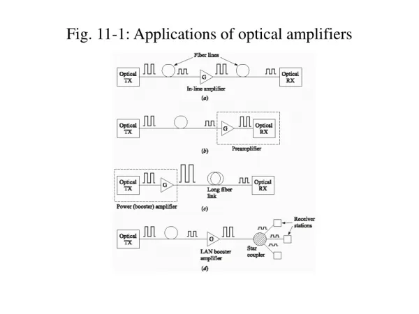
5.1.5. Amplifier Applications • Power amplifier/booster to boost the power transmitted • In-line amplifiers to replace electronic regenerator, but limited by the cumulative effects of fiber dispersion, fiber nonlinearity and amplifier noise. • Optical preamplifier to improve the receiver sensitivity • Distribution amplifier to compensate distribution loss in LAN
5.2 Semiconductor Optical Amplifiers 5.2.1. Amplifier Design • Fabry-Perot amplifier: gain spectrum and its amplifier bandwidth • The condition of TW-type SOA
5.2 Semiconductor Optical Amplifiers 5.2.2. Amplifiers Characteristics • Peak gain increases linearly with the carrier population N: g(N) = (Gsg/V)(N-No) where, G: the confinement factor, sg: the differential gain V: the active volume, No: the value of N required at transparency • Carrier population/photon number dN/dt = I/q – N/tc – Psg(N-No)/smhn = 0 for steady state
5.2.2. Amplifiers Characteristics • The saturated gain g = go/(1 + P/Ps) where, small signal gain go = (Gsg/V)(Itc/q - No) saturation power Ps = hnsm/(sgtc) • Noise figure including internal losses (absorption & scattering) Fn = 2[N/(N-No)][g/(g-aint)] ~ 5-7dB • The polarization sensitivity from the different gain between TE and TM modes. (Dg ~ 5-8dB)
5.2 Semiconductor Optical Amplifiers 5.2.3. Pulse Amplification • The amplification factor is shape dependent, implying distortion • Saturation-induced SPM and the associated frequency chirp
5.2.3. Pulse Amplification • The frequency chirp is opposite compared with that imposed by directly modulated semiconductor lasers. • The amplified pulse would pass through an initial compression stage when it propagates in the anomalous-dispersion region of optical fiber • The compression mechanism can be used to design fiber-optic communication systems in which in-line SOAs are used to compensate simultaneously for both fiber loss and dispersion by operating SOAs in the saturation region • The gain of each bit in an SOA depends on the bit pattern. This phenomenon be quite problematic for WDM systems in which several pulse trains pass through the amplifier simultaneously.
5.2 Semiconductor Optical Amplifiers 5.2.4. System Application • Preamplifier-- degrading the SNR through spontaneous-emission noise. Fn = 5-7 dB • Power amplifier-- too low saturation power ~ 5mW • In-line amplifier-- polarization sensitive, inter-channel crosstalk, large coupling losses • Possible applications (1) wavelength conversion (2) fast switch for wavelength routing in WDM networking (3) low-cost fiber amplifier for metropolitan-area network
5.3 Raman Amplifier 5.3.1. Introduction • Stimulated Raman scattering(SRS) • The incident pump photon gives up its energy to create another photon of reduced energy at a lower frequency (inelastic scattering); the remaining energy is absorbed by the medium in the form of molecular vibration (optical phonons) • The pump and signal beams counter-propagate in the backward-pumping configuration commonly used in practice. • The gain peaks at a Stoke shift of about 13.2 THz. • The gain bandwidth Dng is about 6 THz by FWHM • The large BW makes fiber Raman amplifier attractive • Large pump power: Pp = 5W for 1-km-long fiber, when gR = 6 x 10-14 m/W, λ=1.55 mm, ap= 50 mm
5.3 Raman Amplifier 5.3.2. Raman Gain and Bandwidth • gR/ap, a measure of Raman-gain efficiency • Raman Spectrum from SiO2 fiber
5.3.3 Raman Amplifier Characteristics • Small-signal amplification factor GA & small-signal gain go, When apL>>1 go = gR(Po/ap)(Leff/L) ~ gRPo/apapL GA = Ps(L)/[Ps(0)exp(-asL)] = exp(goL) =exp(gogRPo/apap) where Po = Pp(0) ap is the loss coefficient of pump L is the amplifier length. • Noise from spontaneous Raman scattering, but is neglected because of the distributed nature of the amplification
5.3.4. Raman Amplifier Performance • Raman amplifier can provide 20-dB gain at a pump power of ~1 W. • The broad width of Raman amplifiers is useful for amplifying several channels simultaneously (dense WDM) • Lumped Raman amplifier: a discrete device is made by spooling 1-2 km of an especially prepared fiber that has been doped with Ge or P for enhancing the Raman gain. • Distributed Raman amplifier: the same fiber that is used for signal transmission is also used for signal amplification.
5.3.4. Raman Amplifier Performance • Compact high-power semiconductor and fiber lasers make Raman amplifiers competitive to EDFA. • Rayleigh scattering limits the performance of distributed Raman amplifiers. • The crosstalk accumulates over multiple amplifiers, it can lead to large power penaltiesfor undersea lightwave system with long lengths.
5.3.4 Raman Amplifier Performance • With multiple pump lasers at different wavelengths, the gain spectrum of Raman amplifier is flattened to suit for WDM system.
5.4 Erbium-Doped Fiber Amplifiers 5.4.1. Introduction 5.4.2. Pumping Requirement 5.4.3. Gain Spectrum 5.4.4. Simple Theory 5.4.5. Amplifier Noise 5.4.6. Multi-channel Amplification 5.4.7. Distributed-Gain Amplifiers
5.4 Erbium-Doped Fiber Amplifiers 5.4.1. Introduction • Typical Operating Wavelength Region • Conventional Band (C band) 1530nm ~ 1560nm • Long Band (IR or L band) 1575 nm ~ 1605 nm • OA need one or more pump laser: many pump wavelengths are available (980 nm and 1480 nm most commonly used) • Erbium is the key of optical amplification due to its unique characteristics (EDFA = Erbium Doped Fiber Amplifier) • Amplified Spontaneous Emission (ASE) is broad band noise
5.4 Erbium-Doped Fiber Amplifiers TRANSITION EXCITED STATE METASTABLE STATE STIMULATED PHOTON 1550 nm PUMP PHOTON 980 nm SIGNAL PHOTON 1550 nm FUNDAMENTAL STATE FUNDAMENTAL STATE
5.4.2. Pumping Requirement • The amorphous nature of silica broadens the energy levels of Er+ into bands. • Efficient EDFA pumping is possible using semiconductor lasers operating near 0.98- and 1.48-mm wavelengths. • Efficiencies as high as 11 dB/mW were achieved by 1990 with 0.98-mm pumping. • Most EDFAs use 980-nm pump lasers as such lasers are commercially available and can provide more than 100mW of pump power. • Pumping at 1480 nm requires longer fibers and higher powers because it uses the tail of the absorption band.
5.4.2. Pumping Requirement • In the saturation regime, the power-conversion efficiency is generally better in the backward-pumping configuration, mainly because of the important role played by the amplified spontaneous emission (ASE) • Bidirectional pumping has the advantage that the population inversion, and hence the small-signal gain, is relatively uniform along the entire amplifier length.
5.4.3. Gain Spectrum • The gain spectrum of erbium ions alone is homogeneously broadened. • The gain spectrum of EDFA doped with Ge is quite broad and has a double-peak structure. The addition of Al to the fiber core broadens the gain spectrum even more. • The gain spectrum of alumino-silicate glasses has roughly equal contributions from homogeneous and inhomogeneous broadening mechanisms, contributing up to 35 nm. • The gain spectrum of EDFA depends on the amplifier length because both the absorption and emission cross sections having different spectral characteristics. • The local inversion or local gain varies along the fiber length because of pump power variations. • The total gain is obtained by integrating over the amplifier length.
5.4 Erbium-Doped Fiber Amplifiers 5.4.4. Simple Theory of EDFAs • A three-level rate-equation model commonly used for lasers can be adapted for EDFAs. • A simple two-level model is valid when ASE and excited-state absorption are negligible. • The pump and signal powers vary along the amplifier length because of absorption, stimulated emission, and spontaneous emission. If the contribution of ASE is neglected,
5.4.4. Simple Theory of EDFAs • The total amplifier gain G for an EDFA of length L • A 35-dB gain can be realized at a pump power of 5 mW for L=30m and 1.48-mm pumping • The output saturation power is about 10-mW. • As single-pulse energy are typically much below the saturation energy (~10mJ), EDFAs respond to the average power. • Gain saturation is governed by the average signal power, and the amplifier gain does not vary from pulse to pulse even for a WDM signal.
5.4.5. Amplifier Noise of EDFAs • For a lumped EDFA, the impact of ASE is quantified through the noise figure Fn given by Fn= 2nsp > 3dB • For three-level pumping, N1≠0, so nsp= N2/(N2-N1)>1 • A noise figure of 3.2dB was measured in a 30-m-long EDFA pumped at 0.98um with 11 mW of power. • It is difficult to achieve high gain, low noise, and high pumping efficiency simultaneously. The main limitation is imposed by the ASE traveling backward toward the pump and depleting the pump power. An internal isolator can reduce this problem. • The measured values of Fn are generally larger for EDFAs pumped at 1.48-mm. The reason is that the pump level and the excited level lie within the same band for 1.48-mm pumping.
5.4.6. Multi-channel Amplification • The cross-gain saturation can be avoided by operation the amplifier in the unsaturated regime. • Due to 10 ms carrier lifetime, the gain of EDFAs can not be modulated (carrier-density modulation) at frequencies much than 10 kHz. • The main limitation of an EDFA stems from the spectral nonuniformity of the amplifier gain. • Even a 0.2-dB gain difference grows to 20 dB over a chain of 100 in-line amplifiers. • The entire BW of 35-40 nm can be used if the gain spectrum is flattened by introducing wavelength-selective losses through an optical filter. • L-band: 1570-1610 nm, C-band: 1530-1570nm, S-band:1470-1520nm
5.4.6. Multi-channel Amplification 2nd Active Stage Counter-pumped 1st Active Stage Co-pumped Er3+ Doped Fiber Er3+ Doped Fiber Output Signal Input Signal Optical Isolator Optical Isolator Optical Isolator PUMP PUMP
5.4 Erbium-Doped Fiber Amplifiers 5.4.7. Distributed-Gain Amplifiers • Lumped amplifier: most EDFAs provide 20-25dB amplification over a length ~10m through a relatively high density of dopants (~500 parts per million) • Distributed amplifier ~ distributed Raman amplifier the transmission fiber itself is lightly doped (dopant density ~ 50 part per billion) to provide the gain distributed over the entire fiber length such that it compensates for fiber loss locally. • Distributed EDFA ~ distributed Raman amplifier except that the dopants provide the gain instead of the nonlinear phenomenon of SRS. • Pumping at 980nm is ruled out due to fiber loss > 1dB/km • Pumping loss > 0.4dB/km for 1480nm • This scheme has not yet been used commercially as it requires special fibers.
5.5 System Applications 5.5.1. Optical Pre-amplification • After 1995, due to low insertion loss, high gain, large BW, low noise, and low crosstalk, EDFAs are used as preamplifier at the receiver. • The receiver sensitivity can be improved by 10-20 dB using an EDFA as a preamplifier. • The most important performance issue in designing optical preamplifier is the contamination of the amplified signal by the ASE. • The receiver sensitivity is Prec = hnFnDf[Q4+Q(Dnopt/Df)1/2] where BER = (1/2)erfc(Q/√2); Dnopt is the BW of the optical filter, and Df is the electrical noise BW of the receiver.
5.5.1. Optical Pre-amplification • The receiver sensitivity is written in terms of the average number of photon/bit, Np, by Prec=Nphn and Df = B/2, Np = (1/2)Fn[Q2+Q(2Dnopt/B)1/2] • It shows clearly why amplifiers with a small noise figure must be used. • It also shows how optical filters can improve the receiver sensitivity by reducing Dnopt • The minimum optical BW is equal to the bit rate to avoid blocking the signal. • For Q = 6 (BER=10-9), Np = 44.5 • Np > 1000 for PIN with amplifier. Np < 100 can be realized when optical amplifiers are used to pre-amplify the signal.
5.5.2. Noise Accumulation in Long-Haul System • The amplifier-induced noise builds up due to the cascaded amplifiers in a long-haul lightwave system • Two disadvantages of ASE noise (1) degrading SNR (2) saturating optical amplifier and reducing the gain of amplifiers located further down the fiber link. (3) self-regulating behavior that the total power obtained by adding the signal and ASE powers remains relatively constant. • Electrical SNR is dominated by the signal-spontaneous beat noise generated at the photodetector SNR = PinLA/(4nsphn0LTexp(aLA)] ~ 20dB when nsp= 1.6, a = 0.2 dB/km, Df =10 Gbps • Typically, LA~ 50km for undersea systems and LA~ 80km for terrestrial systems with link lengths under 3000km.
5.5.2. Noise Accumulation in Long-Haul System • Amplifier-induced noise builds up due to the cascaded amplifiers
5.5.2. Noise Accumulation in Long-Haul System • Self-regulating behavior that the total power obtained by adding the signal and ASE powers remains relatively constant.
5.5.2. Noise Accumulation in Long-Haul System Popt Popt OSNR Link Length • Degradation of OSNR • Noise at Rx l l