Download
1 / 46
460 likes | 570 Views
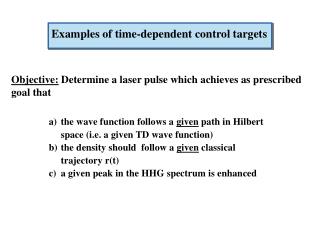
Examples of time-dependent control targets. Objective: Determine a laser pulse which achieves as prescribed goal that. the wave function follows a given path in Hilbert space (i.e. a given TD wave function) the density should follow a given classical trajectory r(t)

E N D
Examples of time-dependent control targets Objective: Determine a laser pulse which achieves as prescribed goal that • the wave function follows a given path in Hilbert space (i.e. a given TD wave function) • the density should follow a given classical trajectory r(t) • a given peak in the HHG spectrum is enhanced
Control the path of the current with laser right lead left lead
Control the path of the current with laser right lead left lead
Optimal control of time-dependent targets OUTLINE THANKS OUTLINE THANKS • Optimal Control Theory (OCT) of static targets • -- OCT of current in quantum rings • -- OCT of ionization • -- OCT of particle location in double well • with frequency constraints • Optimal Control of time-dependent targets • -- OCT of path in Hilbert space • -- OCT of path in real space • -- OCT of harmonic generation Alberto Castro Esa Räsänen Angel Rubio (San Seb) Kevin Krieger Jan Werschnik Ioana Serban
Optimal control of static targets (standard formulation) For given target state Φf , maximize the functional:
Optimal control of static targets (standard formulation) For given target state Φf , maximize the functional: Ô
Optimal control of static targets (standard formulation) For given target state Φf , maximize the functional: Ô with the constraints: E0 = given fluence
Optimal control of static targets (standard formulation) For given target state Φf , maximize the functional: Ô with the constraints: E0 = given fluence
Optimal control of static targets (standard formulation) For given target state Φf , maximize the functional: Ô with the constraints: E0 = given fluence TDSE
Optimal control of static targets (standard formulation) For given target state Φf , maximize the functional: Ô with the constraints: E0 = given fluence TDSE GOAL: Maximize J = J1 + J2 + J3
Set the total variation of J = J1 + J2 + J3 equal to zero: Control equations Algorithm 1. Schrödinger equation with initial condition: Forward propagation Backward propagation New laser field 2. Schrödinger equation with final condition: 3. Field equation: Algorithm monotonically convergent: W. Zhu, J. Botina, H. Rabitz, J. Chem. Phys. 108, 1953 (1998))
Control of currents 2 |y(t)| |y(t)| j (t) j and l = 1 l = -1 l = 0 I ~ mA E. Räsänen, A. Castro, J. Werschnik, A. Rubio, E.K.U.G., PRL 98, 157404 (2007)
OCT of ionization • Calculations for 1-electron system H2+ in 3D • Restriction to ultrashort pulses (T<5fs) • nuclear motion can be neglected • Only linear polarization of laser (parallel or perpendicular to molecular axis) • Look for enhancement of ionization by pulse-shaping only, keeping the time-integrated intensity (fluence) fixed
Control target to be maximized: with Standard OCT algorithm (forward-backward propagation) does not converge: Acting with before the backward-propagation eliminates the smooth (numerically friendly) part of the wave function.
Instead of forward-backward propagation, parameterize the laser pulse to be optimized in the form with ω0 = 0.114 a.u. (λ = 400 nm) with ωn = 2πn/T Choose N such that maximum frequency is 2ω0 or 4ω0 . T is fixed to 5 fs. MaximizeJ1(f1…fN, g1…gN)directly with constraints: using algorithm NEWUOA(M.J.D. Powell, IMA J. Numer. Analysis28, 649 (2008))
of initial pulse of initial pulse Ionization probability for the initial (circles) and the optimized (squares) pulse as function of the peak intensity of the initial pulse. Pulse length and fluence is kept fixed during the optimization.
Control of electron localization in double quantum dots: t = 0 ps t = 1.16 ps t = 2.33 ps t = 3.49 ps t = 4.66 ps t = 5.82 ps E. Räsänen, A. Castro, J. Werschnik, A. Rubio, E.K.U.G., Phys. Rev. B 77, 085324 (2008).
target state: f = first excited state (lives in the well on the right-hand side)
Optimization results Optimized pulse Occupation numbers
E Spectrum OCT finds a combination of several transition processes
algorithm Forward propagation of TDSE (k) Backward propagation of TDSE (k) new field: (W. Zhu, J. Botina, H. Rabitz, J. Chem. Phys. 108, 1953 (1998))
With spectral constraint: filter function: or J. Werschnik, E.K.U.G., J. Opt. B 7, S300 (2005) algorithm Forward propagation of TDSE (k) Backward propagation of TDSE (k) new field: (W. Zhu, J. Botina, H. Rabitz, J. Chem. Phys. 108, 1953 (1998))
E Frequency constraint: Only direct transition frequency 0 allowed occupation numbers Spectrum of optimized pulse
E Frequency constraint: Selective transfer via intermediate state occupation numbers Spectrum of optimized pulse
E Frequency constraint: Selective transfer via intermediate state
Frequency constraint: All resonances excluded occupation numbers Spectrum of optimized pulse
All pulses shown give close to 100% occupation at the end of the pulse
OPTIMAL CONTROL OF TIME-DEPENDENT TARGETS Maximize
Control equations Set the total variation of J = J1 + J2 + J3 equal to zero: Algorithm 1. Schrödinger equation with initial condition: Forward propagation Backward propagation New laser field 2. Schrödinger equation with final condition: Inhomogenous TDSE : 3. Field equation: Y. Ohtsuki, G. Turinici, H. Rabitz, JCP 120, 5509 (2004) I. Serban, J. Werschnik, E.K.U.G. Phys. Rev. A 71, 053810 (2005)
Control of path in Hilbert space with given target occupation, and Goal: Find laser pulse that reproduces |αo(t)|2 I. Serban, J. Werschnik, E.K.U.G. Phys. Rev. A 71, 053810 (2005)
Control path in real space with given trajectory r0(t). Algorithm maximizes the density along the path r0(t): I. Serban, J. Werschnik, E.K.U.G. Phys. Rev. A 71, 053810 (2005) • J. Werschnik and E.K.U.G., in: Physical Chemistry of Interfaces and Nanomaterials V, M. Spitler and F. Willig, eds, Proc. SPIE 6325, 63250Q(1-13) (ISBN: 9780819464040, doi: 10.1117/12.680065); also on arXiv:0707.1874
Control of time-dependent density of hydrogen atom in laser pulse
Control of charge transfer along selected pathways Trajectory 1 Trajectory 2
Time-evolution of wavepacket with the optimal laser pulse for trajectory 1
Trajectory 1: Results Start
Populations of eigenstates ground state first excited state second excited state fifth excited state
Optimization of Harmonic Generation Harmonic Spectrum: Maximize: To optimize the 7th harmonic of ω0, choose coefficients as, e.g., α7= 4, α3 =α5 = α9 = α11 = -1
3 5 7 9 11 13 15 17 19 21 Harmonic generation of helium atom (TDDFT calculation in 3D) Enhancement of 7th harmonic xc functional used: EXX
Thanks ! SFB 450 SFB 658 SPP 1145 Research&Training Network