Download
1 / 36
460 likes | 752 Views
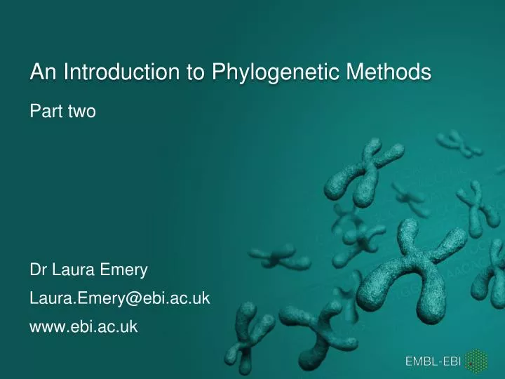
An Introduction to Phylogenetic Methods. Part two. Dr Laura Emery Laura.Emery@ebi.ac.uk www.ebi.ac.uk. Objectives. After this tutorial you should be able to … Discuss a range of methods for phylogenetic inference, their advantages , assumptions and limitations

E N D
An Introduction to Phylogenetic Methods Part two Dr Laura Emery Laura.Emery@ebi.ac.uk www.ebi.ac.uk
Objectives • After this tutorial you should be able to… • Discuss a range of methods for phylogenetic inference, their advantages, assumptionsand limitations • Implement some phylogenetic methods using publicly available software • Appreciate some approaches for assessing branch support and selecting an appropriate substitution model • Know where to look for further information
Outline • Alignment for phylogenetics • Phylogenetics: The general approach • Phylogenetic Methods (1 – simple methods) • Assessing Branch Support BREAK • Substitution Models • Phylogenetic Methods (2 - statistical inference) • Deciding which model to use (hypothesis testing) • Software
The problem of multiple substitutions A * • More likely to have occurred between distantly related species • > We need an explicit model of evolution to account for these hidden mutations * G A * * A T
Methodological approaches • Distance matrix methods (pre-computed distances) • UPGMA assumes perfect molecular clock Sokal & Michener (1958) • Minimum evolution (e.g. Neighbor-joining, NJ) Saitou & Nei (1987) • Maximum parsimony Fitch (1971) • Minimises number of mutational steps • Maximum likelihood, ML • Evaluates statistical likelihood of alternative trees, based on an explicit model of substitution • Bayesian methods • Like ML but can incorporate prior knowledge What is a substitution model?
Statistical phylogenetic inference Figure Brian Moore
Models of sequence evolution • We use models of substitution to ‘roughly’ describe the way that we believe the sequences have evolved • They are necessarily highly simplified descriptions of more complex biological processes • Parameters can be added to build more sophisticated models if we believe this is relevant for our data
Substitution Models • Common nested models • Jukes and Cantor (JC) 1969 • Kimura 2 Parameter (K2P) 1980 • Felsenstein 1981(F81) • Hasegawa, Kishino and Yano 1985 (HKY85) • Generalised time-reversible (GTR or REV) Tavaré1986 • Accounting for rate heterogeneity • Other substitution models
The Jukes and Cantor (JC) 1969 model μ • 1 parameter • μ= mutation rate • Assumptions • Equal base frequencies • All mutations equally likely • All sites evolve at the same rate • All sites evolve independently • Time reversibility A C μ μ μ μ μ μ μ μ μ μ G T μ • d =estimated nucleotide distance • p = observed distance in sequence data
But not all substitutions are equally likely… Transitions are more likely to occur than transversions Figures Andrew Rambaut
Kimura 2 Parameter (K2P) 1980 μ • 2 parameters • μ= mutation rate • κ= transition/transversion ratio • Assumptions • Equal base frequencies • All mutations equally likely • All sites evolve at the same rate • All sites evolve independently • Time reversibility A C μ μ μ κ κ κ κ μ μ μ G T μ • d =estimated nucleotide distance • p = observed distance in sequence data • q= proportion of sites with transversional differences
But base frequencies are often not equal... Base frequencies vary among and within genomes AC T G
Felsenstein 1981 (F81) • πA • πC • 4 symbols (3 parameters) • πA,πC,πG,πT = base frequencies • πA+ πC+ πG +πT = 1(so 3 parameters) • Assumptions • Equal base frequencies • All mutations equally likely • All sites evolve at the same rate • All sites evolve independently • Time reversibility A C G T • πT • πG
Hasegawa, Kishino and Yano 1985 (HKY85) • πA • πC μ • 6 symbols (5 parameters) • μ= mutation rate • κ= transition/transversionratio • πA ,πC,πG,πT = base frequencies • Assumptions • Equal base frequencies • All mutations equally likely • All sites evolve at the same rate • All sites evolve independently • Time reversibility A C μ μ μ κ κ κ κ μ μ μ G T • πT • πG μ
But there are also differences among the other nucleotide transition rates... • A C • A G • A T • C G • C T • G T Figures Andrew Rambaut
Generalised time-reversible (GTR) Tavaré1986 • πA • πC rAC • 10 symbols (9 parameters) • rAC, rAG, rAT, rCG, rCT, rGT= mutation rates • πA,πC,πG,πT = base frequencies • Assumptions • Equal base frequencies • All mutations equally likely • All sites evolve at the same rate • All sites evolve independently • Time reversibility A C rAC rAT rCG rCT rAG rAG rCT rCG rAT rGT G T • πT • πG rGT Widely used
But some sites overall faster than others... 973 mtDNA CR; parsimony analysis (with known pedigree) Heyeret al. (2001)
Gamma distributed rates • Rate variation among sites is often shown to be well-approximated by a gamma distribution • To use: add alpha (α) parameter to existing model e.g. GTR+G • Assumptions • Equal base frequencies • All mutations equally likely • All sites evolve at the same rate • All sites evolve independently • Time reversibility α = 200 0.06 Frequency α = 0.5 0.04 α = 2 α = 50 0.02 0 1 2 Substitution rate
Other substitution models • Amino acid substitution models • Dayhoff 1972 • Whelan and Goldman 2001 (WAG) • Lee & Gascuel 2008 (LG) • Codon models e.g. Yang 2000 • Relaxed molecular clock e.g. Drummond et al. 2006 • Mixture models • And many more!
Methodological approaches • Distance matrix methods (pre-computed distances) • UPGMA assumes perfect molecular clock Sokal & Michener (1958) • Minimum evolution (e.g. Neighbor-joining, NJ) Saitou & Nei (1987) • Maximum parsimony Fitch (1971) • Minimises number of mutational steps • Maximum likelihood, ML • Evaluates statistical likelihood of alternative trees, based on an explicit model of substitution • Bayesian methods • Like ML but can incorporate prior knowledge What is a substitution model?
Statistical phylogenetic inference recommended methods Figure Brian Moore
Maximum Likelihood • Calculate the probability of the observed sequence data under a given model(including tree structure, branch lengths, and transition parameters). [The likelihood is proportional to this probability.] • Search for the tree(s) which maximize(s) the likelihood. model parameters probability data (alignment) Likelihood branch lengths topology constant
Maximum Likelihood • Advantages: • statistically consistent • requires the use of an explicit model of evolution • Disadvantages: • slow (especially if all possible trees are evaluated) • produces a single ML tree • Usage: Widely-used and recommended method recommended
Bayesian Inference • Calculate the probability of the modelspecified given the sequence data observed (using equation derived from Bayes Theorem) • Search the tree-space using MCMC (or equivalent) to approximate the joint-posterior probability density likelihood function prior probability posterior probability marginal likelihood
Bayesian Inference • Advantages: • the option to incorporate prior knowledge • produces probability distribution of possible trees • unlike ML, treats model parameters as random variables • Disadvantages: • very slow • heuristic methods of tree searching do not guarantee you find the best tree • Usage: Widely-used and recommended method recommended
Heuristic searches do not guarantee you find the best tree Figure Andrew Rambaut
Methodological approaches • Distance matrix methods (pre-computed distances) • UPGMA assumes perfect molecular clock Sokal & Michener (1958) • Minimum evolution (e.g. Neighbor-joining, NJ) Saitou & Nei (1987) • Maximum parsimony Fitch (1971) • Minimises number of mutational steps • Maximum likelihood, ML • Evaluates statistical likelihood of alternative trees, based on an explicit model of substitution • Bayesian methods • Like ML but can incorporate prior knowledge What is a substitution model? How do I choose a substitution model?
How do I choose a substitution model? biological intuition develop hypothesis test hypothesis • Identify most appropriate assumptions and thus model for your data • Will a complex model with fewer assumptions better explain your data than a simple model? • Likelihood ratio test • Bayes factor test • Not sure where to start? Empirical data shows GTR+G (nucleotide) or LG (protein) to be a good bet for standard datasets large in size
Choosing a more complex model with more parameters will always fit the data better > We want to know if the fit is significantly better R2= 0.78 R2= 0.86 R2 = 1
Likelihood ratio test • Requires models to be nested • Uses likelihood ratio to evaluate if our hypothesis (H1) is significantly better than our null hypothesis (H0): Likelihood ratio = L(H1)/L(H0) • Twice the logarithm of this ratio (2Δ) approximates a chi-squared distribution under the null hypothesis H0: 2Δ = 2[ln(L(H1)) – ln(L(H0))] • with d degrees of freedom corresponding to the difference in the number of free parameters between models Likelihood of null hypothesis Likelihood of hypothesis Twice the difference in log likelihood Log likelihood of null hypothesis Log likelihood of hypothesis
Likelihood ratio test example • Question: Do the rates of transitions and transversionsin my sequence data significantly vary? • H1: K2P better explains my data (2 rate parameters, transitions different to transversions) • H0: JC is adequate (1 rate parameter for all substitutions) • Draw trees, find out ln(L(K2P)) = -23345; ln(L(JC)) = -23368 • Calculate: 2Δ = 2[ln(L(H1)) – ln(L(H0))] 2Δ= 2[ -23345 - -23368] = 2x23 = 46 • d = difference in number of free parameters = 2 - 1 = 1 • Next we look this up on a Χ2distribution…
Likelihood ratio test example • Is our 2Δ(twice log of the likelihood ratio) greater than we would expect by chance (p = 0.05)? • 2Δ = 46 (d = 1) YES – 46 is much larger than 0.004 > We can reject H0 (JC) and accept H1 (K2P)
Software • And lots lots more see: http://evolution.genetics.washington.edu/phylip/software.html
Outline • Alignment for phylogenetics • Phylogenetics: The general approach • Phylogenetic Methods (1 – simple methods) • Assessing Branch Support BREAK • Substitution Models • Phylogenetic Methods (2 - statistical inference) • Deciding which model to use (hypothesis testing) • Software
Now it is your turn… • Open your course manuals and begin Tutorial 2 (page 13) • Also available to download from: http://www.ebi.ac.uk/training/course/scuola-di-bioinformatica-2013 • You will require the alignment file Rodents.txt • You will require the software SeaView 4.4.2 http://pbil.univ-lyon1.fr/software/seaview.html • There are answers available online but it is much better to ask for help!
Thank you! www.ebi.ac.uk Twitter: @emblebi Facebook: EMBLEBI