Download
1 / 19
190 likes | 304 Views
Demonstration and Comparison of Sequential Approaches for Altimeter Data Assimilation in HYCOM. A. Srinivasan, E. P. Chassignet, O. M. Smedstad, C. Thacker, L. Bertino, P. Brasseur, T. M. Chin,, F. Counillon, and J. Cummings. Outline: Assimilation Schemes Twin Experiments Results/Diagnostics.

E N D
Demonstration and Comparison of Sequential Approaches for Altimeter Data Assimilation in HYCOM A. Srinivasan, E. P. Chassignet,O. M. Smedstad,C. Thacker, L. Bertino,P. Brasseur,T. M. Chin,, F. Counillon, and J. Cummings. Outline: Assimilation Schemes Twin Experiments Results/Diagnostics
Sequential assimilation schemes for HYCOM 1.Optimal Interpolation 2. Multivariate Optimal Interpolation (J. Cummings, O.M. Smedstad –NRL) 3. Ensemble Optimal Interpolation & Kalman Filter (F. Counillon, L. Bertino – NERSC) 4. Ensemble Reduced Order Information Filter (T. M. Chin, Univ of Miami/JPL) 5. Singular Evolutive Extended Kalman Filter (P. Brasseur – LEGI, Grenoble)
Multivariate Optimal InterpolationNRL Coupled Data Assimilation System (NCODA) • Oceanographic version of MVOI method used in NWP systems (Daley, 1991) • Simultaneous analysis of five ocean variables: temperature, salinity, geopotential, and u-v velocity components (T, S, F, u, v) Observation Space Formulation where xais the analysis xb is the background Pb is the background error covariance R is the observation error covariance H is the forward operator (spatial interpolation) (xa – xb)is the analyzed increment [y-H(xb)] is the innovation vector(synoptic T, S, u, v observations)
Ensemble Optimal Interpolation (ENOI) • Covariance are based on an historical ensemble composed of 3 year 10 day model output (106 members) without assimilation • Covariance are 3D multivariate • Conservation of the dynamical balance of the model since the update is a linear combination of model state • Temporal invariance of the covariance matrix, computationally cheap Xa = Xf + A’A’THT ( HA’A’T HT + o o)-1 (Y- HXf) Kalman Gain obs-model X : model state (, t, s, u, v, thk); (a: analysis; f: forecast) A’: centered collection of model states (A’=A-A) Y : observations H : interpolates from model grid to observation o : Observation error : rebalance ensemble variability to realistic level
Ensemble Reduced Order Information Filter (ENROIF) • The ROIF assimilation scheme parameterizes the covariance matrix using a second-order Gaussian Markov Random Field (GMRF) model • A sparse auto-regression operator operates • on the error in the MRF neighborhood • ej = i€Zαijej-i + νj • The square of the regression operator is the • Information Matrix which is the inverse of • the covariance Matrix • Recently replaced the extended KF with ensemble methods to propagate the information matrix. • Uses a static Information matrix generated using 55 members in all experiments shown here MRF order 2 Neighborhood
Gulf of Mexico Model Configuration • Configuration: • 89° to 98°W Longitude and 8° to 31°N Latitude • 1/12 horizontal grid (258x175 pts; 6.5km average spacing) • 20 vertical layers • Forcing from NOGAPS/FNMOC 1999-2000 • Monthly River Runoff • Nested within 1/12 N. Atlantic domain • HYCOM V. 2.1.36
Sequential Analysis-Forecast-Analysis Cycle Ocean Obs Innovations SST: Ship, Buoy, AVHRR(GAC/LAC), GOES, AMSR-E, AATSR, MSG SSH: Altimeter (Jason, Envisat, GFO), in situ Temp/Salt profiles Assimilation Schemes Restart Files GOM HYCOM First Guess Communication via restart files