Download
1 / 47
480 likes | 1.39k Views
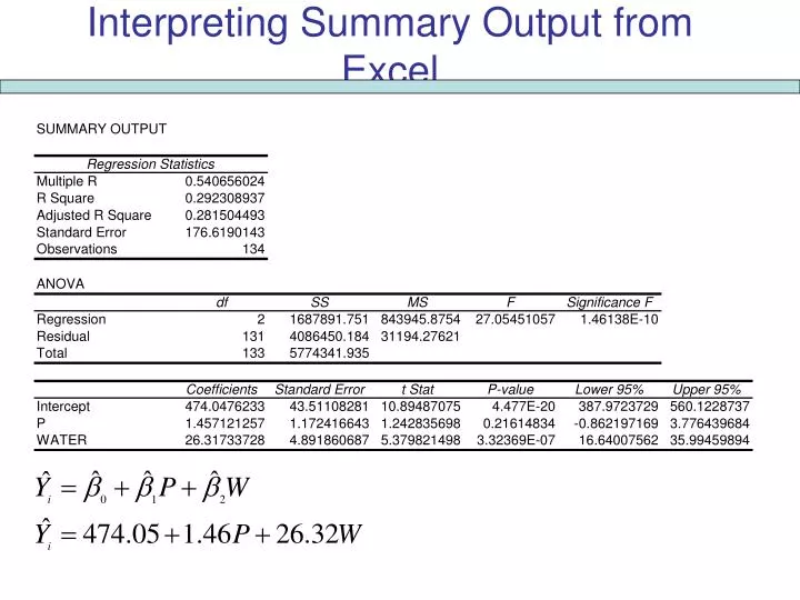
Interpreting Summary Output from Excel. Interpreting Summary Output from Excel. Regression Statistics. Multiple R. 0.540656024. Multiple R: The correlation between Y i and Ŷ i is 54.1%. Interpreting Summary Output from Excel. Regression Statistics. Multiple R. 0.540656024. R Square.

E N D
Interpreting Summary Output from Excel Regression Statistics Multiple R 0.540656024 Multiple R: The correlation between Yi and Ŷi is 54.1%
Interpreting Summary Output from Excel Regression Statistics Multiple R 0.540656024 R Square 0.292308937 29.23% of the variation in Cotton Lint Yields is explained by the independent variables: P & W
Interpreting Summary Output from Excel Regression Statistics Multiple R 0.540656024 R Square 0.292308937 Adjusted R Square 0.281504493 Used to test if an additional independent variable improves the model.
Interpreting Summary Output from Excel Regression Statistics Multiple R 0.540656024 R Square 0.292308937 Adjusted R Square 0.281504493 Standard Error 176.6190143 The Standard Error is the error you would expect between the predicted and actual dependent variable. Thus, 176.62 means that the expected error for a cotton lint yield prediction is off by 176.62 lbs/ac.
Interpreting Summary Output from Excel Regression Statistics Multiple R 0.540656024 R Square 0.292308937 Adjusted R Square 0.281504493 Standard Error 176.6190143 Observations 134
AAEC 4302ADVANCED STATISTICAL METHODS IN AGRICULTURAL RESEARCH Chapter 12: Hypothesis Testing
Statistical Hypothesis Testing • Two complementary hypotheses: • Null hypothesis – H0 • Alternative hypothesis – H1 • Three sets of hypotheses: H0 : Bj = Bj0 H1 : Bj ≠ Bj0 H0 : Bj = Bj0 H1 : Bj > Bj0 H0 : Bj = Bj0 H1 : Bj < Bj0
Statistical Hypothesis Testing • Basic significance test: H0 : Bj = 0 H1 : Bj ≠ 0 • Decision rule: Reject H0 if Reject H0 Do not reject H0 Reject H0 <- - - - - - -І- - - - - - - - - І - - - - - - - - -І - - - - - - - > 0
Statistical Hypothesis Testing • 2 types of mistakes: H0 is true H0 is false (H1 is false) (H1 is true) ______________________________________ Reject H0 Error – Type I Correct decision ______________________________________ Do not Correct Error – Type II Reject H0 decision
Statistical Hypothesis Testing • Consider test statistics defined as: • Decision rule: Reject H0 if • Linear transformation that yields a random variable Z that has a normal distribution (μ=0, σ=1) • Critical value Zc is determined from Pr(ІZІ≥Zc)=α
Statistical Hypothesis Testing • T-statistics is defined as • Decision rule: Reject H0 if
Statistical Hypothesis Testing • To calculate k+1 t-statistics: • ; where is the value of estimated using the OLS formulas and is any “assumed” true (population) value of
Statistical Hypothesis Testing • The t-statistics are used to test the “null’ hypothesis that the true unknown population value of Bj is equal to its assumed true population value (above) • The tests are conducted based on the fact that if the “null” hypothesis is correct, the corresponding t-statistic follows a t distribution with n-k-1 degrees of freedom
Statistical Hypothesis Testing • The t-statistics are also included in the Excel output • Why use a t test, instead of a z test? • Need 100+ observations to use a Z test, thus, we usually use the t, regardless of the number of observations.
Statistical Hypothesis Testing Example: Yi = B0 + B1X1 + B2X2 + Ui Ŷi = B0 + B1X1 + B2X2 Ŷi = 474.05 + 1.46X1 +26.32X2 Where: Yi = Cotton Yields (lbs/ac) X1 = Phosphorous Fertilizer (lbs/ac) X2 = Irrigation Water (in/ac) ^ ^ ^
Statistical Hypothesis Testing ^ P(Bi) Assume: B1 = 1.50 S.E.1 = σ(B1) = 1.20 B1~N(B1, σ2) => ~N(1.50, 1.202) ^ ^ B1 B1=1.50 ^ B1=1.46
Statistical Hypothesis Testing ^ P(Bi) Assume: B1 = 0 S.E.1 = σ(B1) = 1.20 B1~N(B1, σ2) => ~N(0, 1.202) ^ ^ B1 B1=0 ^ B1=1.46
Statistical Hypothesis Testing What can we conclude about ? Since 1.46 is inside the probability distribution, we cannot be certain that is not zero.
Statistical Hypothesis Testing ^ P(B2) Assume: B2 = 0 S.E.1 = σ(B2) = 5 B2~N(B2, σ2) => ~N(0, 52) ^ ^ B2=26.32 ^ B2 B2=0 3σ=15
Statistical Hypothesis Testing is clearly outside the distribution. Therefore, is likely not to belong to this distribution, i.e. is likely not to be equal to zero.
Statistical Hypothesis Testing • Strictly speaking, the t-statistics are only valid under the following additional conditions: • The error term follows a normal distribution with a zero mean and a constant variance for all n observations, i.e.: • A zero mean occurs if no relevant independent variables are left out of the multiple regression model
Statistical Hypothesis Testing • The dependent variable follows a normal distribution with a constant variance across observations • The values taken by the dependent variable in different observations are not correlated to each other • If Ui (and thus Yi) are not normally distributed, the t-statistics are roughly valid if the sample is large enough (more than 250 observations)
Statistical Hypothesis Testing • The steps of the t-statistic is to test: • State the hypotheses • Choose the level of significance α • Calculate the value of the test statistics t* • Find a “critical” value from table (Table A.3 ) • Apply the decision rule
Statistical Hypothesis Testing • In practice, values are typically 0.10, 0.05 or 0.01, depending on the nature and objectives of the research: • these indicate three possible levels of statistical certainty when rejecting H0 (90, 95 and 99%)
Statistical Hypothesis Testing • The decision rule is: • If |tj*| ≥ critical t-table value (at desired and n-k-1 degrees of freedom), reject H0 and: • Conclude that Bj is statistically different from zero • Conclude that Xj affects Y with a certainty level of (1-)
Statistical Hypothesis Testing • The decision rules are: In a one-tailed alternative: • H0 is the same • Ha: Bj< 0 • The decision rule is: If tj*≤ critical t-table valuereject H0
Some General Remarks • When reporting the results of a regression analysis, it is customary to report either the standard errors or the t-values in parenthesis below the corresponding parameter estimate. • Ŷi = 474.05 + 1.46X1 +26.32X2 (43.511)*** (1.172) (4.892)*** Where: * Significant at the 90% level, i.e. α=0.10 ** Significant at the 95% level, i.e. α=0.05 *** Significant at the 99% level, i.e. α=0.01
Some General Remarks • It is also customary to always conduct a “basic” test for the statistical significance of each of the model’s parameters: • test: H0: Bj=0 for j=1,…,k
Statistical Hypothesis Testing Example: Ŷi = 474.05 + 1.46X1 +26.32X2 Where: Yi = Cotton Yields (lbs/ac) X1 = Phosphorous Fertilizer (lbs/ac) X2 = Irrigation Water (in/ac)
Statistical Hypothesis Testing Ŷi = 474.05 + 1.46X1 +26.32X2based on 134 observations Question: Is B1=0? Test: H0: B1 = 0 Ha: B1≠ 0 (two-tailed test)
Statistical Hypothesis Testing Ŷi = 474.05 + 1.46X1 +26.32X2Two-tailed test: t*1 = ( -B1)/(S.E.) = (1.457-0)/(1.172) = 1.243 df = (n - k -1) = (134 - 2 - 1) = 131 Next we must find tc from Table A.3 Using an α=0.10 and df ≈ 125 we find tc≈ 1.657
Statistical Hypothesis Testing P(t) (α/2) = 0.50 (α/2) = 0.50 t 0 -1.657 -tc 1.243 t*1 1.657 tc
Statistical Hypothesis Testing • Since: |t*1|<tc, 1.243<1.657 • We cannot reject the null hypothesis (H0), for α=0.10 (two-tailed test) and df=131.
Statistical Hypothesis Testing Ŷi = 474.05 + 1.46X1 +26.32X2based on 134 observations Question: Is B1=0? Test: H0: B1 = 0 Ha: B1> 0 (one-tailed test)
Statistical Hypothesis Testing Ŷi = 474.05 + 1.46X1 +26.32X2One-tailed test: t*1 = ( -B1)/(S.E.) = (1.457-0)/(1.172) = 1.243 df = (n - k -1) = (143 - 2 - 1) = 131 Next we must find tc from Table A.3 Using an α=0.10 and df ≈ 125 we find tc≈ 1.288
Statistical Hypothesis Testing P(t) t 0 1.243 t*1 1.288 tc
Statistical Hypothesis Testing • Since: |t*1|<tc, 1.243<1.288 • We cannot reject the null hypothesis (H0), for α=0.10 (two-tailed test) and df=131.
Some General Remarks • A “rule of thumb” is that: • If |Bj|>2S[Bj] (i.e. |tj*|>2) • Bj is statistically different from zero, at least at the 95% level of statistical certainty. (=0.05 level of statistical significance) ^ ^
Some General Remarks • One-tail test vs. two-tail test Advantage • If you properly justify that Xj has only a positive (negative) effect on the dependent variable Yi, then the one-tail test will help you reject the null hypothesis. • Under a one-tail test, the critical t-value is smaller than the critical t-value under a two-tail test.
Some General Remarks • One-tail test vs. two-tail test Disadvantage • If you decide that Xj has only a positive effect on Y, than you cannot change your decision after running the regression.
Some General Remarks • Two-tail test vs. one-tail test Advantage • It is more flexible than the one-tailed test because Xj can have either a positive or negative effect on Y.
Some General Remarks • Two-tail test vs. one-tail test Disadvantage • It is more difficult to reject the null hypothesis (H0).