Download
1 / 48
480 likes | 622 Views
The Pre-Industrial European Climate What were the dominant mechanisms?. Lennart Bengtsson with Kevin Hodges ESSC, Reading and Erich Roeckner Renate Brokopf MPI, Hamburg.

E N D
The Pre-Industrial European ClimateWhat were the dominant mechanisms? Lennart Bengtsson with Kevin Hodges ESSC, Reading and Erich Roeckner Renate Brokopf MPI, Hamburg Lennart Bengtsson MPI f Met, Hamburg ESSC, Reading
What do we know about European climate variations?In this study we will focus on surface temperature ( 2m above ground) • This is probably the best observed part of the world. • Several meteorological stations with daily records back to the middle of the 18th century • A few observational records back to the 17th century. • Documentary proxy evidence of incidental character ( e.g. Brazdil et al., 2005 with references) • Sea ice data ( Baltic Sea and Iceland), Greenland ice core, tree ring evidence from Scandinavia etc. • We have here used recent data sets compiled by Luterbacher (2005) Lennart Bengtsson MPI f Met, Hamburg ESSC, Reading
What are the processes leading to climate variations? • Internal variations of the climate system • ( Hasselmann, 1976, Manabe and Stouffer, 1996) • Volcanic aerosols warming the stratosphere and cooling the troposphere • Solar variations in addition to the 11-year cycle • Anthropogenic influences (GHG and aerosols, land surface changes) Lennart Bengtsson MPI f Met, Hamburg ESSC, Reading
What do we know about the causes to European climate variations? • Anthropogenic effects have increasingly influenced climate since the early 20th century, but presumably not so much before that time. • Volcanic aerosols have influenced climate, but only for a few years at most • Solar variability is still an open issue, no variations except the 11-year cycle according to recent summary of satellite records (Frölich, 2005) • We know that climate varies due to internal processes such as ENSO. Lennart Bengtsson MPI f Met, Hamburg ESSC, Reading
Lennart Bengtsson MPI f Met, Hamburg ESSC, Reading
Why have we done this study now? • The latest model at MPI (ECHAM5/MPI-OM) have demonstrated features which we believe are important. These include: • Realistic portraying of ENSO ( Oldenborgh et al., 2005) • A good simulation of tropical intra-seasonal variability(Lin et al., 2005) • Realistic simulation of extra-tropical and tropical storm tracks( Bengtsson et al., 2005) • Long stable integration without the use of flux adjustment • Relatively high resolution ( T63/L31) • Recent compilation of satellite records indicate that there is no discernible trend in TSI (total solar irradiance) 1978-2005 ( Frolich, 2005) and that the empirical relation between sun spots and TSI is not any longer obvious. Consequently previously compiled data sets of long term variation in TSI and used by modelers could be put into question. Long-term TSI trend has been reassessed (2005) and significantly reduced. Lennart Bengtsson MPI f Met, Hamburg ESSC, Reading
TSI (1978-2005) After C Frolich (2005)ISSI, Bern Lennart Bengtsson MPI f Met, Hamburg ESSC, Reading
Assessment of long-term variation in TSI • Judith Lean ( PAGES News, Vol 13, No.3) • “ stellar data has been reassessed, instrumental drifts are suspected in the aa-index, and it has been shown that the long-term trends in the aa-index and cosmogenic isotopes do not neccessarily imply equivalent long-term trends in solar irradiance” • In the latest synthesis by Wang, Lean and Sheeley, 2005 (Astrophys. J.625, 522-538) has the amplitude in low frequency irradiation been reduced to 0.27x Lean 2000. • This means a difference between the Maunder Minimum and the present TSI of only 0.5 Wper m2 ) or 0.09W effectively. Lennart Bengtsson MPI f Met, Hamburg ESSC, Reading
Is it at all possible to reconstruct the evolution of the regional climate? • Ensemble integrations with GCMs show generally large differences between individual members. • Exceptions can be found in some regions in relation to ENSO events. ( but then ENSO must be known) • The European region is under influence of Atlantic storm tracks which are only weakly constrained by external or remote forcing. • Reconstruction of climate evolution is closely related to climate predictability ( of the 1st kind) Lennart Bengtsson MPI f Met, Hamburg ESSC, Reading
St. Petersburg prediction 10.1 2006 17th onward ca -30 C Lennart Bengtsson MPI f Met, Hamburg ESSC, Reading
IPCC AR4 Arctic Temperature Anomalies by AOGCMs 20th Century (20C3M) 11/20 models have decadal signal Courtesy, J Overland PIcntrl (Control Runs) 10/20 models have decadal signal Lennart Bengtsson MPI f Met, Hamburg ESSC, Reading
The pre-industrial European climate 1500-1900.Some science issues • What is the typical internal variability? • How is the variability related to global variability? • Over which periods can trends be observed? • What are the characteristic features of extreme events? • How are the storm tracks related to climate anomalies? • What is the relation to NAO, PNA and ENSO? Lennart Bengtsson MPI f Met, Hamburg ESSC, Reading
Reconstruction of climate from observations • Upper air • 1978 until present global 3D-reconstruction • 1947 until 1978 global reconstruction feasible, but significant errors for SH and the tropics • Surface only • Late 19th century until present surface observations for a major part of the globe • 19th century climate observations from selected regions • 18th century small number of selected observations • 17th century and earlier (essentially only indirect information) Lennart Bengtsson MPI f Met, Hamburg ESSC, Reading
Reconstruction of climate from observations and proxy data • Global, hemispheric, 1000-2000, annual resolution • Mann et al, 1999 • Jones and Mann, 2004 and references therein • Europe (1500-2003, seasonal resolution) • Luterbacher et al., 2004 • Xoplaki et al., 2005 • Luterbacher et al., 2005 ( this study) Lennart Bengtsson MPI f Met, Hamburg ESSC, Reading
Luterbacher, Science 2004 Lennart Bengtsson MPI f Met, Hamburg ESSC, Reading
Luterbacher Science 2004 Lennart Bengtsson MPI f Met, Hamburg ESSC, Reading
Warmest and coldest season in Europe 1500-2003 Luterbacher et al(2004), Xoplaki et al (2005) Lennart Bengtsson MPI f Met, Hamburg ESSC, Reading
The Luterbacher (2005) data set compared to Luterbacher et al., (2004) • Gridded data from Mitchell and Jones (2005) • Additional instrumental predictors mainly from 18th and 19th century • Additional proxies for the 1500-1650 period Lennart Bengtsson MPI f Met, Hamburg ESSC, Reading
Observed winter (JJA) temperature for Europe 1500-2000Luterbacher 2005 * -0.1 -5.7 Lennart Bengtsson MPI f Met, Hamburg ESSC, Reading
Observed summer (JJA) temperature for Europe 1500-2000Luterbacher 2005 +18.2 +15.6 Lennart Bengtsson MPI f Met, Hamburg ESSC, Reading
Global annual averaged temperature500-year integration with ECHAM/MPI-OMPre-industrial atmospheric composition. No variation in external or internal forcing +14.6 Climate drift 0.027/cent. +13.7 Lennart Bengtsson MPI f Met, Hamburg ESSC, Reading
The pre-industrial climate compared to the present (90- year mean) • Atmospheric composition • CO2: 286.2 ppm ( now 382 ppm) ( 1960-1990 ~ 350 ppm) • CH4: 805.6 ppb • N2O: 276.7 ppb • No CFCs • Surface temperature effect: • Global - 0.19 K • European land area winter - 0.54 K • European land area summer ~0 Lennart Bengtsson MPI f Met, Hamburg ESSC, Reading
Model simulation of el Nino/la Nina (NINO3 index) during 500 years Lennart Bengtsson MPI f Met, Hamburg ESSC, Reading
Model simulation of the North Atlantic Oscillation (NAO)during 500 years Lennart Bengtsson MPI f Met, Hamburg ESSC, Reading
Lennart Bengtsson MPI f Met, Hamburg ESSC, Reading
Storm tracks at high NAO ( >2 sd, left) and low NAO( < 2 sd, right) Intensity and density (top)and generation (below) Lennart Bengtsson MPI f Met, Hamburg ESSC, Reading
50-year trends>0.23 corresponds to 95% significance T Sea ice Z 850 P Lennart Bengtsson MPI f Met, Hamburg ESSC, Reading
50-year sea-ice trend>0.23 corresponds to 95% significance * * Lennart Bengtsson MPI f Met, Hamburg ESSC, Reading
Model winter (DJF) temperature for Europe during 500 years +1.5 - 7.5 Lennart Bengtsson MPI f Met, Hamburg ESSC, Reading
Pre-industrial temperatures in Europe (DJF)Model results ( smaller numbers in right column are observed values prior to 1950 covering ca 200 years Lennart Bengtsson MPI f Met, Hamburg ESSC, Reading
Observed winter (JJA) temperature for Europe 1500-2000Luterbacher 2005 * 1500 1900 Lennart Bengtsson MPI f Met, Hamburg ESSC, Reading
Model summer (JJA) temperature for Europe during 500 years 19.1 15.6 Lennart Bengtsson MPI f Met, Hamburg ESSC, Reading
Pre-industrial temperatures in Europe (JJA)Model results ( smaller numbers in right column are observed values prior to 1950 covering ca 200 years Lennart Bengtsson MPI f Met, Hamburg ESSC, Reading
Observed summer (JJA) temperature for Europe 1500-2000Luterbacher 2005 +18.2 * +15.6 1500 1900 Lennart Bengtsson MPI f Met, Hamburg ESSC, Reading
Observation and model statisticsLuterbacher et al., 2005 ( Temp. in C) Lennart Bengtsson MPI f Met, Hamburg ESSC, Reading
Coldest winter and warmest summerleft observed, right model 1941/42 1947 Lennart Bengtsson MPI f Met, Hamburg ESSC, Reading
Lennart Bengtsson MPI f Met, Hamburg ESSC, Reading
Observation and model statisticsLuterbacher et al., 2005 ( Temp. in C) Lennart Bengtsson MPI f Met, Hamburg ESSC, Reading
Ten coldest European wintersmodel and “observations”( Luterbacher, 2005) Model Obs Model global anomaly Model height 500 hPa Lennart Bengtsson MPI f Met, Hamburg ESSC, Reading
Ten warmest European summersmodel and “observations”( Luterbacher, 2005) Model Observ. Lennart Bengtsson MPI f Met, Hamburg ESSC, Reading
Largest temperature differences between 30 year periodswinter ( cold-warm) left, summer (warm-cold) right model observ. Model global Lennart Bengtsson MPI f Met, Hamburg ESSC, Reading
Coldest-warmest winterWarmest-coldest summerLargest 30 - year averages Lennart Bengtsson MPI f Met, Hamburg ESSC, Reading
SummaryPre-industrial European climate over 500 years ( land area) • There is a good agreement between modeled and “observed” winter and summer temperature • Modeled variance is slightly higher than observed but agreement better in the 19th century • The coldest winter in the model is colder than observations and the warmest summer is warmer than observed. There are considerably similarities with observed extreme seasons. • The ten coldest winters are associated with a warmer central tropical Pacific and a warmer Arctic • The ten warmest summers are associated with colder than normal tropical oceans • Sustained anomalies over 30 years in the model experiment are similar to observations but observed summer anomalies are larger Lennart Bengtsson MPI f Met, Hamburg ESSC, Reading
SummaryPre-industrial European climate over 500 years ( land area) • Global temperature anomalies is well correlated with ENSO (0.70 in DJF) • There is virtually no correlation between global temperature anomalies and European temperature anomalies. • As in observations modeled European winter temperature is correlated with NAO (0.46) • There are regional trends on the time scale of 50 years( significant at 95%) Lennart Bengtsson MPI f Met, Hamburg ESSC, Reading
ConclusionsThe European climate 1500-1900 • It is strongly suggested that that the climate of Europe during the period was strongly dominated by natural variability and that external forcing ( total solar irradiance, TSI and volcanic aerosols) only have had a minor effect. • This is supported by the fact that extreme temperature for different seasons occur at very different times. For example the coldest summer and autumn occurred in the beginning of the 20th century, while the coldest winter and spring occurred during the 17th and 18th century respectively. • We believe it is probably not feasible to attribute climate variations in the European region to variations in the external forcing as these variations are completely dominated by internal climate variations • We believe great care must be applied in attribution studies during this period as incorrect conclusions may result when model variance have deficiencies. It is important to recognize that seasons with extreme temperature and even longer periods with unusual temperatures may just happen by chance Lennart Bengtsson MPI f Met, Hamburg ESSC, Reading
Caveats • External forcing from volcanic aerosols ( This is likely to give higher variance during the summer) • Variation in cloudiness due to CCN of cosmic origin • Land-surface changes • Model artifacts Lennart Bengtsson MPI f Met, Hamburg ESSC, Reading
Proposals for further work • Ensemble integrations ( minimum 3) • Extend assessment to other parts of the Earth with long observational records of good quality • Including volcanic aerosols • Including land surface processes • Including orbital forcing Lennart Bengtsson MPI f Met, Hamburg ESSC, Reading
END Lennart Bengtsson MPI f Met, Hamburg ESSC, Reading