Download
1 / 21
270 likes | 603 Views
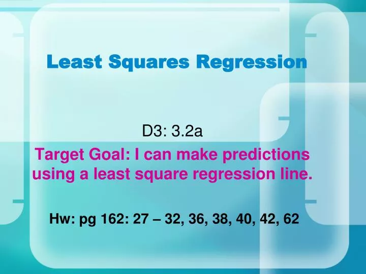
Least Squares Regression. D3: 3.2a Target Goal: I can make predictions using a least square regression line. Hw: pg 162: 27 – 32, 36, 38, 40, 42, 62. LSRL: least squares regression line. a model for the data a line that summarizes the two variables

E N D
Least Squares Regression D3: 3.2a Target Goal: I can make predictions using a least square regression line. Hw: pg 162: 27 – 32, 36, 38, 40, 42, 62
LSRL: least squares regression line • a model for the data • a line that summarizes the two variables • It makes the sum of the squares of the vertical distances of the data points as small as possible
LSRL • The LSRL makes the sum of the squares of these distances as small as possible. The LSRL minimizes the total area of the squares.
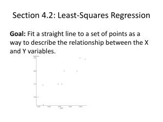
Regression Line • Straight line • Describes how theresponse variable y changes as the explanatory variable x changes. • Use regression line to predictvalue of y for given value of x. • Regression (unlike correlation) requires both an explanatory and response variable.
The dashed line shows how to use the regression line to predict. • You can find the vertical distance of each point on the scatterplot from the regression line.
Predictions and Error • We are interested in the vertical distance of each point on the scatterplot from the regression line. • If we predict 4.9, and the actual value turns out to be 5.1, our error is the vertical distance. Error (residual) = observed y – predicted ŷ
Equation of the least squares regression line • We have data on an explanatory variable x and a response variable y for n individuals. • From the data, calculate the means x bar, y bar,sx,syof the two variables, and their correlation r.
The Least Squares Regression Line (LSRL): • with slope, b = • and intercept, a = y – b ŷ = a + bx
ŷ = a + bx • y: the observed value • ŷ: the predicted value • every LSRL passes through • slope: rate of change We will usually not calculate by hand, we will use the calculator.
Exercise: Gas Consumption • The equation of the regression line of gas consumption y on the degree-days xis: ŷ = 1.0892 + 0.1890x
Verifyingŷ = 1.0892+0.1890x • Use your calculator to find the mean and standard deviation of both x and y and their correlation r from data in the following table.
x bar = = 22.31 • Sx = = 17.74 • y bar = = 5.306 • Sy = = 3.368 • r = 0.99526
Using what we’ve found, find the slope b and intercept a of the regression line from these. b = 0.1890 a = 1.0892 • This Verifies ŷ = 1.0892+0.1890x except for round off error.
Least squares lines on the calculator • Use the same data you entered into L1 and L2. (Turn off other plots & graphs.) • Define the scatterplot using L1 and L2 and the use ZoomStat to plot.
Press STAT:CALC:(8)LinReg(a+bx):L1,L2,Y1:enter To enter Y1, VARS:Y-VARS:(1)FUNCTION} If r2 and r do not appear on your screen, press 2nd:0 (catalog). Scroll down to “DiagnosticOn” and press enter.
Press GRAPH to overlay the LSRL on the scatterplot. • Note: verify LSRL equation at Y1 to be ŷ = 1.0892+0.1890x
Interpreting a Regression Line Consider the regression line from the example “Does Fidgeting Keep You Slim?” Identify the slope and y-intercept and interpret each value in context. Least-Squares Regression The slope b = -0.00344 tells us that the amount of fat gained is predicted to go down by 0.00344 kg for each added calorie of NEA. The y-intercept a = 3.505 kg is the fat gain estimated by this model if NEA does not change when a person overeats.
Prediction We can use a regression line to predict the response ŷfor a specific value of the explanatory variable x. Use the NEA and fat gain regression line to predict the fat gain for a person whose NEA increases by 400 cal when she overeats. Least-Squares Regression We predict a fat gain of 2.13 kg when a person with NEA = 400 calories.
Interpreting Computer Regression Output A number of statistical software packages produce similar regression output. Be sure you can locate • the slope b, • the y intercept a, • and the values of s and r2. Least-Squares Regression
The slope b = -2.9935 tells us that the amount of Pctis predicted to go down by 2.9935 units for each additional pair. The y-intercept a = 157.68 is the Pct estimated by this model when there are no pairs.