Cost Comparison of SKA Antenna Stations John D. Bunton , CSIRO TIP

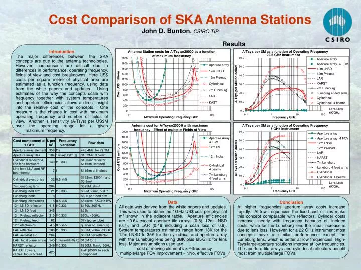
1. Cost Comparison of SKA Antenna StationsJohn D. Bunton, CSIRO TIP Results Introduction The major differences between the SKA concepts are due to the antenna technologies. However, comparisons are difficult due to differences in performance, operating frequency, fields of view and cost breakdowns. Here US$ costs per square metre of physical area are estimated as a function frequency, using data from the white papers and updates. Using estimates of the way the concepts scale with frequency together with system temperatures and aperture efficiencies allows a direct insight into the relative cost of the concepts. One measure is the change in cost with maximum operating frequency and number of fields of view. Another is sensitivity (A/Tsys) per US$M over the operating range for a given maximum frequency. Data All data was derived from the white papers and updates. This was used to obtain the 1GHz US$ cost per physical m2 shown in the adjacent table. Aperture efficiencies are ~0.64 except aperture tile arrays (0.8), 12m LNSD (0.7), and LAR (0.48 including a scan loss of 0.8). System temperatures estimates range from 18K for the 12m LNSD to 35K for the cylindrical and aperture array with the Luneburg lens being 38K plus 6K/GHz for lens loss. Major assumptions used are cost of moving elements  3√frequency multiple/large FOV improvement = √No. effective FOVs Conclusion At higher frequencies aperture array costs increase rapidly. At low frequencies the fixed cost of tiles make this concept comparable with reflectors. Cylinder costs increase linearly with frequency because of linefeed costs, while for the Luneburg lens the linear increase is due to lens loss. However, for a 22 GHz instrument most concepts have a similar performance except the Luneburg lens, which is better at low frequencies. High-Tsys/large-aperture solutions improve at low frequencies. The aperture tile arrays and cylindrical reflectors benefit most from multiple/large FOVs.