Download
1 / 69
690 likes | 711 Views
Sections 6.7, 6.8, 7.7 ( Note : The approach used here to present the material in these sections is substantially different from the approach used in the textbook.).

E N D
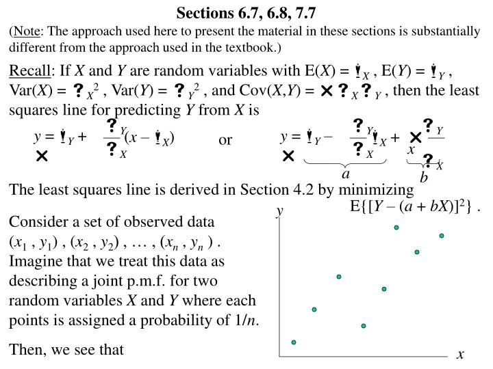
Sections 6.7, 6.8, 7.7 (Note: The approach used here to present the material in these sections is substantially different from the approach used in the textbook.) Recall: If X and Y are random variables with E(X) = X, E(Y) = Y , Var(X) = X2 , Var(Y) = Y2 , and Cov(X,Y) = XY , then the least squares line for predicting Y from X is Y — (x – X) X Y — X + X Y — x X y = Y + y = Y – or a b The least squares line is derived in Section 4.2 by minimizing E{[Y – (a + bX)]2} . y Consider a set of observed data (x1 , y1) , (x2 , y2) , … , (xn , yn ) . Imagine that we treat this data as describing a joint p.m.f. for two random variables X and Y where each points is assigned a probability of 1/n. Then, we see that x
n plays the role of E(X) = X, plays the role of E(Y) = Y , plays the role of Var(X) = X2 , plays the role of Var(Y) = Y2 , and plays the role of Cov(X,Y) = XY . 1 — n x xi = i= 1 n 1 — n y yi = i= 1 n 1 — n n – 1 —— n sx2 (xi– x)2 = i= 1 n 1 — n n – 1 —— n sy2 (yi– y)2 = i= 1 we shall complete this equation shortly. n 1 — n (xi– x)(yi–y) = i= 1
n (xi– x)(yi–y) We define the sample covariance to be c = , and we define the sample correlation to be r = Consequently, the least squares line for predicting Y from X is This least squares line minimizes i= 1 n– 1 c —— . sxsy The sample correlation r is a measure of the strength and direction of a linear relationship for the sample in the same way that the correlation is a measure of the strength and direction of a linear relationship for the two random variables X and Y.
n plays the role of E(X) = X, plays the role of E(Y) = Y , plays the role of Var(X) = X2 , plays the role of Var(Y) = Y2 , and plays the role of Cov(X,Y) = XY . 1 — n x xi = i= 1 n 1 — n y yi = i= 1 n 1 — n n – 1 —— n sx2 (xi– x)2 = i= 1 n 1 — n n – 1 —— n sy2 (yi– y)2 = i= 1 n 1 — n n – 1 —— c n (xi– x)(yi–y) = i= 1
n (xi– x)(yi–y) We define the sample covariance to be c = , and we define the sample correlation to be r = Consequently, the least squares line for predicting Y from X is This least squares line minimizes i= 1 n– 1 c —— . sxsy sy — (x – x) sx sy — x + sx sy r— x sx y = y + r y = y – r or a b n [yi– (a + bxi)]2 . i= 1 The sample correlation r is a measure of the strength and direction of a linear relationship for the sample in the same way that the correlation is a measure of the strength and direction of a linear relationship for the two random variables X and Y.
r = +1 r close to +1 r is positive r is negative r = –1 r close to –1 r close to 0 r close to 0 r close to 0 r is negative
Suppose Y1 , Y2 , … , Yn are independent with respective N(1 , 2), N(2 , 2), … , N(n , 2) distributions. Let x1 , x2 , … , xn be fixed values not all equal, and suppose that for i = 1, 2, …, n, i = 0 + 1xi . Then the joint p.d.f. of Y1 , Y2 , … , Yn is n [yi– (0 + 1xi)]2 – ———————— 22 [yi– (0 + 1xi)]2 – ——————— 22 n i = 1 exp —————————— = 2 exp ———————————— n (2)n/2 i= 1 for – < y1 < , – < y2 < , … , – < yn < If we treat this joint p.d.f. as a function L(0 , 1), that is, a function of the unknown parameters 0 and 1 , then we can find the maximum likelihood estimates for 0 and 1 by maximizing the function L(0 , 1). It is clear the function L(0 , 1) will be maximized when is minimized. n [yi– (0 + 1xi)]2 i= 1
The previous result concerning the least squares line for predicting Y from X with a sample of data points tells us that the mle of 1 is 1 = and the mle of 0 is 0 = n n (xi– x)(Yi–Y) (xi– x)Yi ^ Sy R — = sx = = i= 1 i= 1 n n (xi– x)2 (xi– x)2 i= 1 i= 1 n (xi– x) Yi n i= 1 (xj– x)2 j= 1 x ^ n Yi — n n (xi– x) Sy — x = sx Y – R – = Yi n i= 1 i= 1 (xj– x)2 j= 1 x (xi– x) n 1 — n – Yi n i= 1 (xj– x)2 j= 1
1. (a) Suppose we are interested in predicting a person's height from the person's length of stride (distance between footprints). The following data is recorded for a random sample of 5 people: Length of Stride (inches) 14 13 21 25 17 Height (inches) 61 54 63 72 59 Find the equation of the least squares line for predicting a person's height from the person's length of stride. 120 —— = 1.2 . 100 The slope of the least squares line is The intercept of the least squares line is 61.8 – (1.2)(18) = 40.2 . The least squares line can be written y = 40.2 + 1.2x .
(b) Suppose we assume that the height of humans has a normal distribution with mean 0 + 1x and variance 2, where x is the length of stride. Find the maximum likelihood estimators for 0 and 1 . 120 —— = 1.2 . 100 The mle of 1 is The mle of 0 is 61.8 – (1.2)(18) = 40.2 .
2. (a) Suppose Y1 , Y2 , … , Yn are independent with respective N(1 , 2), N(2 , 2), … , N(n , 2) distributions. Let x1 , x2 , … , xn be fixed values not all equal, and suppose that for i = 1, 2, …, n, i = 0 + 1xi . Use Theorem 5.5-1 (Class Exercise 5.5-1) to find the distribution of the maximum likelihood estimator of 1. ^ n (xi– x) 1 = has a normal distribution with Yi n i= 1 (xj– x)2 j= 1 n n (xi– x) (xi– x) (0 + 1xi) = [0 + 1x + 1(xi – x)] = mean n n i= 1 i= 1 (xj– x)2 (xj– x)2 j= 1 j= 1 n n n (xi– x) (xi– x) (xi– x)2 [0 + 1x] + 1(xi – x) = 1 n n n i= 1 i= 1 i= 1 (xj– x)2 (xj– x)2 (xj– x)2 j= 1 j= 1 j= 1 = 1
2 n n (xi– x) (xi– x)2 2 = 2 and variance = 2 n n i= 1 i= 1 (xj– x)2 (xj– x)2 j= 1 j= 1 2 n (xi– x)2 i= 1
2. - continued (b) Use Theorem 5.5-1 (Class Exercise 5.5-1) to find the distribution of the maximum likelihood estimator of 0. ^ x (xi– x) n 1 — n 0 = has a normal distribution with – Yi n i= 1 (xj– x)2 j= 1 x (xi– x) n 1 — n mean (0 + 1xi) = – n i= 1 (xj– x)2 j= 1 x (xi– x) n 1 — n n (0 + 1xi) – (0 + 1xi) = n i= 1 i= 1 (xj– x)2 We already found this in part (a). j= 1 n (xi– x) (0 + 1xi) = 0 + 1x– x n i= 1 (xj– x)2 j= 1
0 + 1x– 1x = 0 2 x (xi– x) n 1 — n 2 and variance = – n i= 1 (xj– x)2 j= 1 x x2 2 (xi– x) n (xi– x)2 1 — n2 2 = – + 2 n n n i= 1 (xj– x)2 (xj– x)2 j= 1 j= 1 x2 1 — n 2 + n (xi– x)2 i= 1
Suppose we treat the joint p.d.f. as a function L(0 , 1 , 2), that is, a function of the three unknown parameters (instead of just two). Then, analogous to Text Example 6.1-3, we find that the maximum likelihood estimates for 0 and 1 are the same as previously derived, and that the maximum likelihood estimator for 2 is n ^ ^ [Yi– (0 + 1xi)]2 i= 1 n Recall: If Y1 , Y2 , … , Yn are independent with each having a N(, 2) distribution (i.e., a random sample from a N(, 2) distribution), then Y = has a distribution, has a distribution, and n Yi 2 — n N( , ) i= 1 n (n – 1)S2 ———– 2 2(n – 1)
(n – 1)S2 ———– 2 the random variables Y and are independent. Analogous results for the more general situation previously considered can be proven using matrix algebra. Suppose Y1 , Y2 , … , Yn are independent with respective N(1 , 2), N(2 , 2), … , N(n , 2) distributions. Let x1 , x2 , … , xn be fixed values not all equal, and suppose that for i = 1, 2, …, n, i = 0 + 1xi . Then 1 has a distribution, 0 has a distribution, 2 ^ N( 1 , ) n (xi– x)2 i= 1 x2 ^ 1 — n N( 0 , ) 2 + n (xi– x)2 i= 1
n ^ ^ [Yi– (0 + 1xi)]2 2(n – 2) i= 1 has a distribution, random variables and are independent, and random variables and are independent. 2 n ^ ^ [Yi– (0 + 1xi)]2 ^ i= 1 1 2 n ^ ^ [Yi– (0 + 1xi)]2 ^ i= 1 0 2
^ ^ ^ For each i = 1, 2, …, n, we define the random variable Yi = 0 + 1xi , that is, Yi is the predicted value corresponding to xi . With appropriate algebra, it can be shown that ^ ^ n n n (Yi– Y)2 = (Yi– Y)2 + (Yi–Yi)2 i= 1 i= 1 i= 1 This is called the total sum of squares and is denoted SST. This is called the regression sum of squares and is denoted SSR. This is called the error (residual) sum of squares and is denoted SSE. Since, as we have noted, SSE / 2 has a 2(n – 2) distribution, we say that the df (degrees of freedom) associated with SSE is n – 2 . If Y1 , Y2 , … , Yn all have the same mean, that is, if 1 = 0, thenSST / 2 has a 2(n – 1) distribution; consequently, the df associated with SST is n – 1 . If Y1 , Y2 , … , Yn all have the same mean, that is, if 1 = 0, then it can be shown that SSR and SSE are independent, and that SSR / 2 has a 2(1) distribution; consequently, the df associated with SSR is 1 .
3. Suppose Y1 , Y2 , … , Yn are independent with respective N(1 , 2), N(2 , 2), … , N(n , 2) distributions. Let x1 , x2 , … , xn be fixed values not all equal, and suppose that for i = 1, 2, …, n, i = 0 + 1xi . Prove that SST = SSR + SSE . ^ ^ ^ ^ First, we observe that for i = 1, 2, …, n, Yi = 0 + 1xi = Y+ 1(xi – x) 2 ^ ^ n n (Yi– Y)2 = 1(xi–x) + (Yi– Y) – 1(xi – x) = SST = i= 1 i= 1 ^ ^ n [1(xi–x)]2 + [(Yi– Y) – 1(xi – x)]2+ i= 1 ^ ^ 21(xi–x)[(Yi– Y) – 1(xi – x)] = ^ ^ n n [1(xi–x)]2 + [Yi– Y– 1(xi – x)]2 + i= 1 i= 1 n ^ n ^ 2 1(xi–x)(Yi– Y) – 12(xi – x)2 = i= 1 i= 1
^ ^ n n (Yi– Y)2 + (Yi–Yi)2 + i= 1 i= 1 ^ ^ n n 2 1 (xi–x)(Yi– Y) – 12 (xi – x)2 = i= 1 i= 1 SSR + SSE + 2 n n (xi– x)(Yi–Y) (xi– x)(Yi–Y) n n 2 (xi–x)(Yi– Y) – (xi–x)2 i= 1 i= 1 2 n n (xi– x)2 (xi– x)2 i= 1 i= 1 i= 1 i= 1 = SSR + SSE
A mean square is a sum of squares divided by its degrees of freedom. SSE —— n – 2 The error (residual) mean square is MSE = . SSR —— 1 The regression mean square is MSR = . Variation in Y explained by the linear relationship with X is based on SSR. Total variation in Y is based on SST. y Variation in Y explained by random error is based on SSE.
If Y1 , Y2 , … , Yn all have the same mean, that is, if 1 = 0, then E(SSR / 2) = and E If 1 0, then E(SSR / 2) = 1 SSE / 2 ——— = n– 2 1 . ^ ^ n n (Yi– Y)2 [1(xi–x)]2 i= 1 i= 1 E ————— = 2 E —————– = 2 n n (xi–x)2 (xi–x)2 ^ ^ ^ E(12) = Var(1) + [E(1)]2 = i= 1 i= 1 ———— 2 ———— 2 n (xi–x)2 1 + 12 > 1 . i= 1 ———— 2
SSE / 2 ——— n– 2 This suggests that if 1 = 0, then the ratio of SSR / 2 to is expected to be close to one, but if 1 0, then this ratio is expected to be larger than one. If 1 = 0, then since SSR and SSE are independent, then the ratio of SSR / 2 to must have an distribution. SSE / 2 ——— n– 2 f( , ) 1 n – 2 Consequently, we can perform the hypothesis test H0: 1 = 0 vs. H1: 1 0 . by using the test statistic F = We reject H0 (in favor of H1) when The linear relationship (correlation) between X and Y is not significant. The linear relationship (correlation) between X and Y is significant. SSR / 2 ———— = MSR ——– . MSE SSE / 2 ——— n– 2 f > f(1, n– 2) .
The calculations in a regression leading up to the f statistic are often organized into an analysis of variance (ANOVA) table such as the following: 1 SSR MSR MSR / MSE n– 2 SSE MSE n– 1 SST It can be shown that the squared sample correlation is R2 = which is often called the proportion of variation in Y explained by X. The standard error of estimate is defined to be SXY = SSR —— . SST (This is done in Class Exercise #7.) MSE .
1. - continued (c) Find the sums of squares SSR, SSE, and SST; then construct the ANOVA table and perform the corresponding f test with = 0.05, find and interpret the squared sample correlation, and find the standard error of estimate. ^ ^ n n SSR = (Yi– Y)2 = 12 (xi–x)2 = (1.2)2(100) = 144 i= 1 i= 1 n SST = (Yi– Y)2 = 174.8 i= 1 SSE = SST– SSR = 174.8– 144 = 30.8
1 144 144 14.03 0.025< p < 0.05 3 30.8 10.267 4 174.8 Since f = 14.03 > f0.05(1,3) = 10.13, we reject H0. We conclude that the slope in the linear regression of height on stride length is different from zero (0.025< p-value < 0.05), and the results suggest that this slope is positive. (Note: We could alternatively conclude that the linear relationship or correlation is significant, and that the results suggest a positive linear relationship or correlation.) R2 = 144 / 174.8 = 82.4% of the variation in height is explained by stride length. The standard error of estimate is SXY = 10.267 = 3.20 inches.
8. (a) The prediction of grip strength from age for right-handed males is of interest. It is assumed that for any age x in years, where 10 x 25, Y = “grip strength in pounds” has a N(x , 2) distribution where x = 0 + 1x. For a random sample of right-handed males, the following data are recorded: Age (years) 15 17 19 11 16 22 17 25 12 14 25 23 Grip Strength (lbs.) 50 54 66 46 58 54 64 80 46 70 76 80 Obtain the calculations below from a calculator and from SPSS. n = 12 x = 18 y = 62 n n (yi– y)2 = (xi– x)2 = 256 1728 i= 1 i= 1 n (xi–x)(yi– y) = 512 r = + 0.770 i= 1
8. - continued (b) (c) Find the equation of the least squares line from a calculator and from SPSS. ^ 1 = 0 = 2 ^ The least squares line can be written y = 26 + 2x . ^ 26 Write a one-sentence interpretation of the slope in the least squares line and a one-sentence interpretation of the intercept in the least squares line. Grip strength appears to increase on average by about 2 pounds with each increase of one year in age. The intercept is the mean grip strength at age zero, which makes no sense in this situation.
(d) (e) Find r2, and write a one-sentence interpretation. r2 = 0.593 About 59.3% of the variation in grip strength is explained by age. Find the standard error of estimate. s = 8.390
8. - continued (f) Construct the ANOVA table and perform the corresponding f test with = 0.05. ^ ^ n n SSR = (Yi– Y)2 = 12 (xi–x)2 = (2)2(256) = 1024 i= 1 i= 1 n SST = (Yi– Y)2 = 1728 i= 1 SSE = SST– SSR = 1728 – 1024 = 704 1 1024 1024 14.55 p < 0.01 10 704 70.4 11 1728 The test statistic is f = 14.55
The critical region with = 0.05 is f 4.96 . The p-value is smaller than 0.01 (from the table) or p = 0.003 (from the SPSS output). 0 4.96 = f0.05(1,10) Since f = 14.55 > f0.05(1,10) = 4.96, we reject H0. We conclude that the slope in the linear regression of grip strength on age is different from zero (p < 0.01), and the results suggest that this slope is positive. (Note: We could alternatively conclude that the linear relationship or correlation is significant, and that the results suggest a positive linear relationship or correlation.)
4. Suppose Y1 , Y2 , … , Yn are independent with respective N(1 , 2), N(2 , 2), … , N(n , 2) distributions. Let x1 , x2 , … , xn be fixed values not all equal, and suppose that for i = 1, 2, …, n, i = 0 + 1xi . Show that the maximum likelihood estimator of 2 is not unbiased; then, find a constant multiple of this maximum likelihood estimator which is an unbiased estimator of 2. n ^ ^ n ^ ^ [Yi– (0 + 1xi)]2 [Yi– (0 + 1xi)]2 2 — n 2 — (n – 2) n E = E = i= 1 i= 1 n 2 n ^ ^ [Yi– (0 + 1xi)]2 n —— n– 2 An unbiased estimator of 2 is = i= 1 n ^ n (Yi–Yi)2 SSE —— = n – 2 = MSE i= 1 ————— n– 2
^ 1 – 1 ^ 1 – 1 = n MSE (xi– x)2 n (xi– x)2 i= 1 SSE / 2 ——— n – 2 i= 1 has a distribution. t(n – 2) ^ ^ 0 – 0 0 – 0 = x2 x2 1 — n 1 — n MSE + + n n (xi– x)2 (xi– x)2 SSE / 2 ——— n – 2 i= 1 i= 1 has a distribution. t(n – 2)
5. Suppose Y1 , Y2 , … , Yn are independent with respective N(1 , 2), N(2 , 2), … , N(n , 2) distributions. Let x1 , x2 , … , xn be fixed values not all equal, and suppose that for i = 1, 2, …, n, i = 0 + 1xi . For a given value x0 , use Theorem 5.5-1 (Class Exercise 5.5-1) to find the distribution of Y | x0 = 0 + 1x0 (the predicted value of Y corresponding to the value x0). ^ ^ ^ ^ (xi– x) (x0 – x) ^ ^ ^ n Yi — n n Y+ 1(x0 – x) = Y | x0 = 0 + 1x0 = + = Yi n (xj– x)2 i= 1 i= 1 j= 1 (xi– x) (x0 – x) n 1 — n has a normal distribution with + Yi n (xj– x)2 i= 1 j= 1
^ ^ mean E(0 + 1x0) = 0 + 1x0 We can find this with algebra analogous to that in Class Exercise #2(b). 2 (x0 – x) n 1 — n (xi– x) 2 and variance = + n (x0 – x)2 (xj– x)2 1 — n i= 1 2 + n j= 1 (xi– x)2 i= 1 In Class Exercise #2(b), this was just x . In Class Exercise #2(b), this was a minus sign.
^ ^ ^ For a given value x0 , we define Y | x0 = 0 + 1x0 to be the predicted value of Y corresponding to the value x0 ; this predicted value has a (x0 – x)2 1 — n N( , ) 0 + 1x0 2 distribution, and + n (xi– x)2 n ^ ^ i= 1 [Yi– (0 + 1xi)]2 ^ ^ ^ random variables and are independent. Y | x0 = 0 + 1x0 i= 1 2 ^ ^ ^ ^ 0 + 1x0 – (0 + 1x0) 0 + 1x0 – (0 + 1x0) = (x0 – x)2 (x0 – x)2 1 — n 1 — n MSE + + n n (xi– x)2 (xi– x)2 SSE / 2 ——— n – 2 i= 1 i= 1 has a distribution. t(n – 2) We assume min{x1 , x2 , … , xn} x0 max{x1 , x2 , … , xn}, since prediction outside the range of the data may not be valid.
6. (a) Suppose Y1 , Y2 , … , Yn are independent with respective N(1 , 2), N(2 , 2), … , N(n , 2) distributions. Let x1 , x2 , … , xn be fixed values not all equal, and suppose that for i = 1, 2, …, n, i = 0 + 1xi . Derive a 100(1 –)% confidence interval for the slope 1 . ^ 1 – 1 P – t/2(n – 2) t/2(n – 2) = 1 – MSE n (xi– x)2 i= 1 MSE MSE ^ ^ P 1 – t/2(n – 2) 1 1 + t/2(n – 2) n n (xi– x)2 (xi– x)2 i= 1 i= 1 = 1 –
(b) If 1(0) is a hypothesized value for 1 , then derive the test statistic and rejection regions corresponding to the one sided and two sided hypothesis tests for testing H0: 1 = 1(0) with significance level . ^ 1 – 1(0) The test statistic is T = MSE n (xi– x)2 i= 1 For H1: 1 < 1(0) , the rejection region is t– t(n – 2) . For H1: 1 > 1(0) , the rejection region is tt(n – 2) . For H1: 1 1(0) , the rejection region is |t| t/2(n – 2) .
8. - continued (g) Perform the t test for H0: 1 = 0.8 vs. H1: 1 0.8 with = 0.05. ^ 1 – 0.8 2 – 0.8 The test statistic is t = = = 2.288 . MSE 70.4 n 256 (xi– x)2 i= 1 The two-sided critical region with = 0.05 is |t| 2.228 . – 2.228 2.228 = t0.025(10) The p-value is between 0.02 and 0.05 (from the table).
Since t = 2.288 > t0.025(10) = 2.228, we reject H0. We conclude that the slope in the linear regression of grip strength on age is different from 0.8 lbs. (0.02 < p < 0.05), and the results suggest that this slope is greater than 0.8 lbs. (Note: We could alternatively conclude that the average change in grip strength is different from 0.8 lbs. per year, and that this change is greater than 0.8 lbs. per year.)
8. - continued (h) Considering the results of the hypothesis tests in parts (f) and (g), explain why a 95% confidence interval for the slope in the regression would be of interest. Then find and interpret the confidence interval. Since rejecting H0 in part (f) suggests that the hypothesized zero slope is not correct, and rejecting H0 in part (g) suggests that the hypothesized slope of 0.8 is not correct, a 95% confidence interval will provide us with some information about the value of the slope, which estimates the average change in grip strength with an increase of one year in age. MSE MSE ^ ^ 1 – t/2(n – 2) 1 1 + t/2(n – 2) n n (xi– x)2 (xi– x)2 i= 1 i= 1 70.4 —— 256 2 (2.228) 0.832 and 3.168
We are 95% confident that the slope in the regression to predict grip strength from age is between 0.832 and 3.168 lbs.
6. - continued (c) Derive a 100(1 – )% confidence interval for the intercept 0 . ^ 0 – 0 P – t/2(n – 2) t/2(n – 2) = 1 – x2 1 — n MSE + n (xi– x)2 i= 1 x2 1 — n ^ MSE + P 0 – t/2(n – 2) 0 n (xi– x)2 i= 1 x2 1 — n ^ MSE + 0 + t/2(n – 2) n = 1 – (xi– x)2 i= 1
(d) If 0(0) is a hypothesized value for 0 , then derive the test statistic and rejection regions corresponding to the one sided and two sided hypothesis tests for testing H0: 0 = 0(0) with significance level . ^ 0 – 0(0) The test statistic is T = x2 1 — n MSE + n (xi– x)2 i= 1 For H1: 0 < 0(0) , the rejection region is t– t(n – 2) . For H1: 0 > 0(0) , the rejection region is tt(n – 2) . For H1: 0 0(0) , the rejection region is |t| t/2(n – 2) .
8. - continued (i) Perform the t test for H0: 0 = 0 vs. H1: 0 0 with = 0.05. ^ 0 – 0 The test statistic is t = = x2 1 — n MSE + n (xi– x)2 i= 1 26 – 0 = 2.668 1 — 12 182 —— 256 70.4 + The two-sided critical region with = 0.05 is |t| 2.228 . The p-value is – 2.228 2.228 = t0.025(10) between 0.02 and 0.05 (from the table) or p = 0.024 (from the SPSS output).
Since t = 2.668 > t0.025(10) = 2.228, we reject H0. We conclude that the intercept in the linear regression of grip strength on age is different from zero (0.02 < p < 0.05), and the results suggest that this intercept is positive.
8. - continued (j) Considering the results of the hypothesis test in part (i), explain why a 95% confidence interval for the intercept in the regression would be of interest. Then find and interpret the confidence interval. Since rejecting H0 in part (i) suggests that the hypothesized zero intercept is not correct, a 95% confidence interval will provide us with some information about the value of the intercept. x2 1 — n ^ MSE + 0 – t/2(n – 2) n (xi– x)2 i= 1 0 x2 1 — n ^ MSE + 0 + t/2(n – 2) n (xi– x)2 i= 1
26 (2.228) 1 — 12 182 —— 256 70.4 + 4.288 and 47.712 We are 95% confident that the intercept in the regression to predict grip strength from age is between 4.288 and 47.712 lbs.
6. - continued (e) For a given value x0 , we can call E(Y | x0) = 0 + 1x0 the mean of Y corresponding to the value x0 , and an unbiased estimator of this mean is Y | x0 = 0 + 1x0 (from Class Exercise #5). Derive a 100(1 – )% confidence interval for E(Y | x0) = 0 + 1x0 . ^ ^ ^ ^ ^ 0 + 1x0 – (0 + 1x0) P – t/2(n – 2) t/2(n – 2) = 1 – (x0 – x)2 1 — n MSE + n (xi– x)2 i= 1