Download
1 / 36
360 likes | 702 Views
2009 NDSS. Scalable, Behavior-Based Malware Clustering. Ulrich Bayer ,Paolo Milani Comparetti ,Clemens Hlauschek ,Christopher Kruegel , and Engin Kirda Technical University Vienna University of California , Santa Brabara Institute Eurecom , Sophia Antipolis.

E N D
2009 NDSS Scalable, Behavior-Based Malware Clustering Ulrich Bayer ,Paolo MilaniComparetti ,Clemens Hlauschek ,Christopher Kruegel , and EnginKirda Technical University Vienna University of California , Santa Brabara Institute Eurecom, Sophia Antipolis 2009.10.21 by Mike Hsiao
Outline • Introduction • System Overview • Dynamic Analysis • Behavior Profile • Scalable Clustering • Evaluation • Limitations and Future Work • Related Work
Introduction • Thousands of new malware samples appear each day. • Automatic analysis systems allow us to create thousands of analysis reports. • Now a way to group the reports is needed. We would like to cluster them into sets of malware reports that exhibit similar behavior. • We require automated clustering techniques. • Clustering allows us to • discard reports of samples that have been seen before • guide an analyst in the selection of those samples that require most attention • derive generalized signatures, implement removal procedures that work for a whole class of samples
Scalable, Behavior-Based Malware Clustering • Malware Clustering: Find a partitioning of a given set of malware samples into subsets so that subsets share some common traits (i.e., find “virus families”) • Behavior-Based: A malware sample is represented by its actions performed at run-time. • Scalable: It has to work for large sets of malware samples.
Dynamic Analysis • Based on our existing automatic, dynamic analysis system called Anubis (based on Qemu). • Anubis is a full-system emulator. • Anubis generates an execution trace listing all invokedsystem calls. • In this work, we extended Anubis with: • system call dependencies (Tainting) • control flow dependencies • network analysis (for accurately describing a sample’s network behavior) • Output of this step: Execution trace augmented with taint information and network analysis results.
Dynamic Analysis (cont’d) • The goal is to identify how the program uses information that it obtains from the OS. • Tainting system • We attach (taint) labels to certain interesting bytes in memory and propagate these labels whenever they are copied or otherwise manipulated. • System calls serves as taint source. • I.e., we taint the out-arguments and return values of all system calls.
Dynamic Analysis (cont’d) • Example • 1) get the return value of GetDate, and then it is used in CreateFile call. • 2) a program reads its own code segment might be a worm propagation code. • Record program control flow • identify similarities between programs that perform the same actions • Network • use Bro to analyze the sent/received data to recognize and parse application level protocols.
Extraction Of The Behavioral Profile • In this step, we process the execution trace provided by the ‘dynamic analysis’ step. • Goal: abstract from the system call trace • system calls can vary significantly, even between programs that exhibit the same behavior • remove execution-specific artifacts from the trace • A behavioral profile is an abstraction of the program‘s execution trace that accurately captures the behavior of the binary.
Reasons For An Abstract Behavioral Description • Different ways to read from a file • Different system calls with similar semantics • e.g., NtCreateProcess, NtCreateProcessEx • You can easily interleave the trace with unrelated calls: f = fopen(“C:\\test”); read(f, 1); read(f, 1); read(f, 1); f = fopen(“C:\\test”); read(f, 3); B: A: f = fopen(“C:\\test”); read(f, 1); readRegValue(..); read(f, 1); C:
Elements Of A Behavioral Profile • OS Objects: represent a resource such as a file that can be manipulated via system calls • has a name and a type • OS Operations: generalization of a system call • carried out on an OS object • the order of operations is irrelevant • the number of operations on a certain resource does not matter • Object Dependencies: model dependencies between OS objects (e.g., a copy operation from a source file to a target file) • also reflect the true order of operations • Control Flow Dependencies: reflect how tainted data is used by the program (comparisons with tainted data)
Example: Behavioral Profile src = NtOpenFile(“C:\\sample.exe”); // memory map the target file dst = NtCreateFile(“C:\\Windows\\” + GetTempFilename()); dst_section = NtCreateSection(dst); char *base = NtMapViewOfSection(dst_section); while(len < length(src)) { *(base+len)=NtReadFile(src, 1); len++; } Op | File | C:\sample.exe open:1, read:1 Op | File | RANDOM_1 create:1 Op | Section | RANDOM_1 open:1, map:1, mem_write: 1 Dep | File | C:\sample.exe -> Section | RANDOM_1 read – mem_write
Example: Behavioral Profile src = NtOpenFile(“C:\\sample.exe”); // memory map the target file dst = NtCreateFile(“C:\\Windows\\” + GetTempFilename()); dst_section = NtCreateSection(dst); char *base = NtMapViewOfSection(dst_section); while(len < length(src)) { *(base+len)=NtReadFile(src, 1); len++; } Op | File | C:\sample.exe open:1, read:1 Op | File | RANDOM_1 create:1 Op | Section | RANDOM_1 open:1, map:1, mem_write: 1 Dep | File | C:\sample.exe -> Section | RANDOM_1 read – mem_write
Example: Behavioral Profile src = NtOpenFile(“C:\\sample.exe”); // memory map the target file dst = NtCreateFile(“C:\\Windows\\” + GetTempFilename()); dst_section = NtCreateSection(dst); char *base = NtMapViewOfSection(dst_section); while(len < length(src)) { *(base+len)=NtReadFile(src, 1); len++; } Op | File | C:\sample.exe open:1, read:1 Op | File | RANDOM_1 create:1 Op | Section | RANDOM_1 open:1, map:1, mem_write: 1 Dep | File | C:\sample.exe -> Section | RANDOM_1 read – mem_write
Example: Behavioral Profile src = NtOpenFile(“C:\\sample.exe”); // memory map the target file dst = NtCreateFile(“C:\\Windows\\” + GetTempFilename()); dst_section = NtCreateSection(dst); char *base = NtMapViewOfSection(dst_section); while(len < length(src)) { *(base+len)=NtReadFile(src, 1); len++; } Op | File | C:\sample.exe open:1, read:1 Op | File | RANDOM_1 create:1 Op | Section | RANDOM_1 open:1, map:1, mem_write: 1 Dep | File | C:\sample.exe -> Section | RANDOM_1 read – mem_write
Example: Behavioral Profile src = NtOpenFile(“C:\\sample.exe”); // memory map the target file dst = NtCreateFile(“C:\\Windows\\” + GetTempFilename()); dst_section = NtCreateSection(dst); char *base = NtMapViewOfSection(dst_section); while(len < length(src)) { *(base+len)=NtReadFile(src, 1); len++; } Op | File | C:\sample.exe open:1, read:1 Op | File | RANDOM_1 create:1 Op | Section | RANDOM_1 open:1, map:1,mem_write: 1 Dep | File | C:\sample.exe -> Section | RANDOM_1 read – mem_write
Example: Behavioral Profile src = NtOpenFile(“C:\\sample.exe”); // memory map the target file dst = NtCreateFile(“C:\\Windows\\” + GetTempFilename()); dst_section = NtCreateSection(dst); char *base = NtMapViewOfSection(dst_section); while(len < length(src)) { *(base+len)=NtReadFile(src, 1); len++; } Op | File | C:\sample.exe open:1, read:1 Op | File | RANDOM_1 create:1 Op | Section | RANDOM_1 open:1, map:1, mem_write: 1 Dep | File | C:\sample.exe -> Section | RANDOM_1 read – mem_write
Example: Behavioral Profile src = NtOpenFile(“C:\\sample.exe”); // memory map the target file dst = NtCreateFile(“C:\\Windows\\” + GetTempFilename()); dst_section = NtCreateSection(dst); char *base = NtMapViewOfSection(dst_section); while(len < length(src)) { *(base+len)=NtReadFile(src, 1); len++; } Op | File | C:\sample.exe open:1, read:1 Op | File | RANDOM_1 create:1 Op | Section | RANDOM_1 open:1, map:1, mem_write: 1 Dep | File | C:\sample.exe -> Section | RANDOM_1 read – mem_write
Example: Behavioral Profile src = NtOpenFile(“C:\\sample.exe”); // memory map the target file dst = NtCreateFile(“C:\\Windows\\” + GetTempFilename()); dst_section = NtCreateSection(dst); char *base = NtMapViewOfSection(dst_section); while(len < length(src)) { *(base+len)=NtReadFile(src, 1); len++; } Op | File | C:\sample.exe open:1, read:1 Op | File | RANDOM_1 create:1 Op | Section | RANDOM_1 open:1, map:1, mem_write: 1 Dep | File | C:\sample.exe -> Section | RANDOM_1 read – mem_write
Scalable Clustering • Most clustering algorithms require to compute the distances between all pairs of points => O(n2). • We use LSH (locality sensitive hashing), a technique introduced by Indyk and Motwani, to compute an approximate clustering that requires less than n2 distance computations. • Our clustering algorithm takes as input a set of malware samples where each malware sample is represented as a set of features. • We have to transform each behavioral profile into a feature set first • Consider a and b are two samples. Our similarity measure: Jaccard Index defined as
LSH Clustering • We are performing an approximate, single-linkage hierarchical clustering: • Step 1: Locality Sensitive Hashing • to cluster a set of samples we have to choose a similarity threshold t • the result is an approximation of the true set of all near (as defined by the parameter t) pairs • Step 2: Single-Linkage hierarchical clustering
Evaluating Clustering Quality • For assessing the quality of the clustering algorithm, we compare our clustering results with a reference clustering of the same sample set • since no reference clustering for malware exists, we had to create it first • Reference Clustering: • we obtained a random sampling of 14,212 malware samples that were submitted to Anubis from Oct. 27th 2007 to Jan. 31st 2008 • we scanned each sample with 6 different virus scanners • we selected only those samples for which the majority of the antivirus programs reported the same malware family. This resulted in a total of 2,658 samples. • we manually corrected classification problems
Quantitative Evaluation • We ran our clustering algorithm with a similarity threshold t = 0.7 on the reference set of 2,658 samples. • Our system produced 87 clusters while the reference clustering consists of 84 clusters. • Precision: 0.984 • precision measures how well a clustering algorithm distinguishes between samples that are different • Recall: 0.930 • recall measures how well a clustering algorithm recognizes similar samples T: reference clustering C: authors’ clustering
Comparative Evaluation NCD: Normalized Compression Distance LSH: Locality Sensitive Hashing Exact: all n*n/2 distance are computed
Precision and Recall t The relationship between Precision/Recall and threshold t.
Performance Evaluation • Input: 75,692 malware samples • Previous work by Bailey et al (extrapolated from their results of 500 samples): • Number of distance calculations: 2,864,639,432 • Time for a single distance calculation: 1.25 ms • Runtime: 995 hours (~ 6 weeks) • Our results: • Number of distance calculations: 66,528,049 • Runtime: 2h 18min
More results • 4 largest cluster (account for 86% of all samples) • Allaple.1 (1,289 samples) • a polymorphic worm with ICMP scans • Allaple.2 (717 samples) • exploit the target systems using a wider variety of propagation behavior with DNS lookup • DOS (179 samples) • This cluster contains various DOS malware sample but with similar behavior • GBDialer.j (106 samples) • similar startup actions and system modification with attempting modem dial
More result • Similar register key access to check if anti-virus system is installed. • Compare fixed value with system time. • to launch a specific action at specific time • Wrong cluster (one cluster with 25 samples) • sample crash • cause debugger activate • generate crash report • display popup message
Limitations and Future Work • Trace Dependence • more behavior might be hidden in other execution context. • Evasion • We are not interested in labor-intensive, manual evasion. • We consider adversary who attempts to automatically produce an arbitrary number of mutations of a malware sample in such a way that most such mutations are assigned to different clusters by our tools.
Related Work • Behavioral Analysis • All of them focus on system call analysis. • Dynamic Data Tainting • Recently, dynamic taint analysis has been also used for the automatic analysis of network protocol. • [18] D. Song, “Polylot: Automatic Extraction of Protocol Message Format using Dynamic Binary Analysis,” in CCS 2007. • [43] C. Kruegel, “Automatic Network Protocol Analysis,” in NDSS 2008. • But they focus on protocol format or syntax analysis, not execution behavior.
Conclusions • Novel approach for clustering large collections of malware samples • dynamic analysis • extraction of behavioral profiles • clustering algorithm that requires less than a quadratic amount of distance calculations • Experiments on real-world datasets that demonstrate that our techniques can accurately recognize malicious code that behaves in a similar fashion • Available online: http://anubis.iseclab.org
Example: Behavioral Profile src = NtOpenFile(“C:\\sample.exe”); // memory map the target file dst = NtCreateFile(“C:\\Windows\\” + GetTempFilename()); dst_section = NtCreateSection(dst); char *base = NtMapViewOfSection(dst_section); while(len < length(src)) { *(base+len)=NtReadFile(src, 1); len++; } Op | File | C:\sample.exe open:1, read:1 Op | File | RANDOM_1 create:1 Op | Section | RANDOM_1 open:1, map:1, mem_write: 1 Dep | File | C:\sample.exe -> Section | RANDOM_1 read – mem_write
Coding for Cluster transform into a set of features 1. For each object , and for each operation 2. For each dependence 3. For each label-value comparison 4. For each label-label comparison