Convolution, Impulse Response, Filters

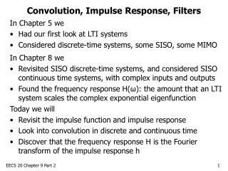
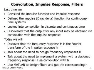
1. Convolution, Impulse Response, Filters Last time we • Revisited the impulse function and impulse response • Defined the impulse (Dirac delta) function for continuous-time systems • Looked into convolution in discrete and continuous time • Discovered that the output for any input may be obtained via convolution with the impulse response Today we will • Discover that the frequency response H is the Fourier transform of the impulse response h • Talk about the need to design frequency responses H • Talk about the need to implement a system with a designed frequency response H via convolution with h • Use MATLAB to design filters and get the corresponding h EECS 20 Chapter 9 Part 2

2. Convolution In Chapter 5, we defined a mathematical operation on discrete-time signals called convolution, represented by  . Given two discrete-time signals x1 , x2  [Integers → Reals], • n  Integers, We can also define convolutions for continuous-time signals. Given two continuous-time signals x1 , x2  [Reals → Reals], • t  Reals, EECS 20 Chapter 9 Part 2

3. Convolution with Impulse Response For both continuous and discrete-time LTI systems, we define the impulse response as the special output that occurs when the input is an impulse function (Dirac delta for continuous-time systems, Kronecker Delta for discrete-time systems). This impulse response, called h, gives us the output for any input via convolution: For x  [Reals → Reals], • t  Reals, For x  [Integers → Integers], • n  Integers, Recall that the roles of h and x in the above may be reversed. EECS 20 Chapter 9 Part 2

4. From Impulse Response to Frequency Response Consider the case when the input to a continuous-time LTI system, x, is an eigenfunction given by x(t) = eiωt. We can find the output y using convolution with the impulse response h: • t  Reals, Recall that an LTI system scales an eigenfunction x(t) = eiωt by a factor H(ω). From above, we see this scaling factor is The frequency response is the Fourier transform of the impulse response. EECS 20 Chapter 9 Part 2

5. From Impulse Response to Frequency Response For the discrete-time case, with x(t) = eiωn for n  Integers, We can find the output y using convolution with the impulse response h: • n  Integers, From above, we see the scaling factor on the eigenfunction is The frequency response is the discrete-time Fourier transform (DTFT) of the impulse response. EECS 20 Chapter 9 Part 2

6. Importance of H and h We want to design systems with a particular frequency response H for many possible applications: • Audio signal correction: getting rid of noise, compensating for an imperfect audio channel (walls that absorb high frequencies) • The equalizer on your stereo lets you modify your stereo’s H • Blurring and edge detection in images: an abrupt change in color in an image indicates high frequency, blocks of constant color are low frequencies • AM radio reception: we want to keep a signal at one particular carrier frequency, and filter out neighboring carrier frequencies Practical implementation of H, at least in digital systems, is easily accomplished by convolution with the corresponding h. EECS 20 Chapter 9 Part 2

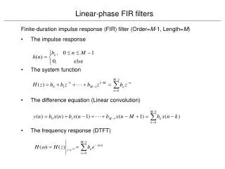
7. Designing FIR Discrete-Time Systems We want to be able to specify a desired frequency response, H(ω) for all ω in Reals, and come up with the corresponding impulse response h(n) for all n in Integers. Our life will be easiest if h(n) is nonzero only for a finite set of samples n  {0, 1, … L-1}. Then the length of the impulse response will be L, and the convolution sum will be finite: So we would like to come up with an FIR implementation of our desired frequency response function H(ω). MATLAB can help. EECS 20 Chapter 9 Part 2

8. Designing FIR Filters Using MATLAB The remez() function in MATLAB implements an algorithm called the Parks-McClellan algorithm based on the Remez algorithm. It comes up with an impulse response of desired length L that implements a bandpass filter minimizing gain in the stopband. You specify the passband, the frequencies your filter should amplify, the stopband, the frequencies it should zero out, and the transition band, the “don’t care” area of transition between 0 and 1. passband stopband EECS 20 Chapter 9 Part 2

9. Designing IIR Discrete-Time Systems Notice that when we were designing our FIR system, with we were really picking the coefficients of a difference equation. We can implement a wider variety of systems with the more general difference equation that involves feedback: These systems may have impulse responses of infinite duration (IIR), and the convolution sum would have infinite terms. So, we design them by selecting the coefficients a and b and implement them using feedback as above. EECS 20 Chapter 9 Part 2

10. Using MATLAB to Design IIR Filters MATLAB has several functions that come up with the difference equation coefficients a and b to implement a system with a desired frequency response H(ω) for all ω in Reals. Using butter() Butterworth filter cheby1() Chebyshev 1 filter cheby2() Chebyshev 2 filter elliptic Elliptic filter you can specify the passband, stopband, and order (number of terms in the difference equation) of your desired H. MATLAB will return the corresponding coefficients in the difference equation. EECS 20 Chapter 9 Part 2

11. Discrete-Time Filter Implementation, Causality We can describe the implementation of filters using block diagrams, which can be implemented in hardware or Simulink. The above diagram illustrates an FIR filter. An IIR filter would add in delayed and scaled versions of y. Note that our filters involve delayed samples x(n-m) where m≥0. The system uses information from the past and present, not the future: no terms with m<0. These systems are called causal. EECS 20 Chapter 9 Part 2

12. Design of Continuous-Time Systems We have just discussed design of discrete-time systems to achieve a particular frequency response by selecting the coefficients of a linear difference equation. To design a continuous-time system with a particular frequency response, we can select coefficients of a linear differential equation. The Butterworth, Chebyshev, and Elliptical methods are famous ways to do this. The differential equation can be implemented using circuits or simulators like Simulink. http://www.maxim-ic.com/appnotes.cfm/appnote_number/1795 EECS 20 Chapter 9 Part 2