Download
1 / 26
290 likes | 624 Views
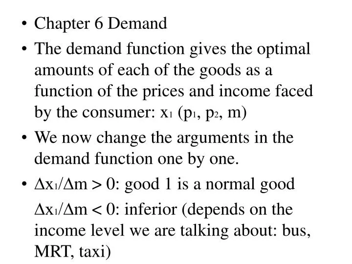
Chapter 6 Demand The demand function gives the optimal amounts of each of the goods as a function of the prices and income faced by the consumer: x 1 (p 1 , p 2 , m) We now change the arguments in the demand function one by one. ∆x 1 /∆ m > 0: good 1 is a normal good

E N D
Chapter 6 Demand • The demand function gives the optimal amounts of each of the goods as a function of the prices and income faced by the consumer: x1 (p1, p2, m) • We now change the arguments in the demand function one by one. • ∆x1/∆m > 0: good 1 is a normal good ∆x1/∆m < 0: inferior (depends on the income level we are talking about: bus, MRT, taxi)
Two ways to look at the same thing • (1) At x1 – x2 space, connect the demanded bundles as the budget line gets shifted outward. This curve is called the income offer curve (IOC) or income expansion path. • (2) At x1 – m space, connect the optimal x1 bundles as the income increases while holding all prices fixed. This curve is called the Engel curve.
Draw a general preference to illustrate the income offer curve and the Engel curve. • Perfect substitutes: p1 < p2, IOC (x axis), Engel (sloped p1) think about p1 > p2 and p1 = p2. • Perfect complements: IOC (at the corner), Engel (sloped p1+ p2) • Cobb-Douglas: x1 = am/ p1 and x2 = (1-a)m/ p2 so x1/x2 is constant, thus IOC (line), Engel (sloped p1/a))
In the above three cases, (∆x1/ x1)/(∆m/m) = 1. They all belong to homothetic preferences. If (x1, x2) w (y1, y2), then for all t >0, (tx1, tx2) w (ty1, ty2). (無異曲線等比例放大縮小)
If (x1, x2) is optimal at m, then (tx1, tx2) is optimal at tm. Suppose not, then (y1, y2) is feasible at tm and (y1, y2) s (tx1, tx2). Then (y1, y2) w (tx1, tx2) and it is not the case that (tx1, tx2) w (y1, y2). However, (y1/t, y2/t) is feasible at m, so (x1, x2) w (y1/t, y2/t). By homothetic preferences, (tx1, tx2) w (y1, y2), a contradiction.
Reasonable? (toothpaste) • Quasilinear preferences: p1 = p2=1, u(x1, x2) = √x1 + x2 • MU1 = 1/(2 √x1), MU2 = 1, MU1/p1 = MU2/p2 implies x1 = ¼ • IOC: on the x-axis up to (1/4,0), then becomes vertical • Engel: sloped 1 up to (1/4, 1/4), then becomes vertical • “zero income effect” only after some point
∆x1/∆p1 > 0: good 1 is a Giffen good ∆x1/∆p1 < 0: good 1 is an ordinary good • Two ways to look at the same thing • (1) At x1 – x2 space, connect the demanded bundles as the budget line gets pivoted outward. This curve is called the price offer curve (POC).
(2) At x1 – p1 space, connect the optimal x1 bundles as own price increases while holding income and other price fixed. This curve is called the demand curve. • Draw a general preference to illustrate the price offer curve and the demand curve.
Perfect substitutes: POC p1 > p2: x1 = 0, p1 = p2: all budget line, p1 < p2: x1 = m/ p1, draw demand curve • Perfect complements: POC (at the corner), demand (m/(p1+p2)) • Discrete: good 1 is in discrete amounts and u(x1, x2) = v(x1) + x2
Suppose m is large enough in the relevant range and let x2 be the amount of money you can spend on all other goods, then you will start to buy the first unit of good 1 when p1 has decreased to v(0)+m = v(1)+m-p1, so p1 has decreased to v(1) – v(0). Similarly, you will start buying the second unit of good 1 when p1 has further decreased to v(1)+m-p1= v(2)+m-2p1, so p1 has decreased to v(2) – v(1). (draw) • Illustrate the demand curve for the quasilinear case
∆x1/∆p2 > 0: good 1 is a substitute for good 2 ∆x1/∆ p2 < 0: good 1 is a complement for good 2 (像自己價格的改變) • The inverse demand function x1= x1 (p1), given p1, how many x1 that a consumer wants to buy p1= p1 (x1), given x1, what price of p1 would have to be in order for the consumer to choose that level of consumption
Cobb Douglas x1 = am/ p1 vs. p1 = am/ x1 • Inverse demand has a useful interpretation |MRS1, 2| = p1/ p2 so p1 = |MRS1, 2| p2 suppose good 2 is the money to spend on all other goods, so p2 = 1 and p1 = |MRS1,2| = ∆$/∆ x1: how many dollars the individual would be willing to give up to have a little more of 1 (marginal willingness to pay)
Demand downward sloping is due to that the marginal willingness to pay decreases as x1 increases (different from diminishing MRS along an indifference curve).