Download
1 / 37
370 likes | 474 Views
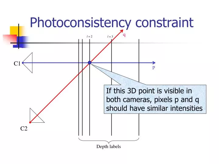
q. l = 2. l = 3. C1. p. If this 3D point is visible in both cameras, pixels p and q should have similar intensities. C2. Depth labels. Photoconsistency constraint. q. l = 2. l = 3. C1. p. Photoconsistency neighbors. C2. Depth labels. Photoconsistency neighborhood.

E N D
q l = 2 l = 3 C1 p If this 3D point is visible in both cameras, pixels p and q should have similar intensities C2 Depth labels Photoconsistency constraint
q l = 2 l = 3 C1 p Photoconsistency neighbors C2 Depth labels Photoconsistency neighborhood
Data (photoconsistency) term • Photoconsistency neighborhood Nphoto • Arbitrary set of pairs of 3D points (same depth) • Current implementation: if the projection of on C2 is nearest to q • Our data penalty for configuration f is • Note that fp = fq=l by definition of Nphoto
Tsukuba images Our results, 4 interactions
Comparison Best results [SS ’02] Our results, 10 interactions
Expectation-Maximization A powerful technique for many computer vision problems
A simple problem – Line fitting • Goal: To group a bunch of points into two “best-fit” line segments
“Chicken-egg problem” • If we knew which line each point belonged to, w could compute the best-fit lines.
Chicken-egg problem • If we knew what the two best-fit lines were, we could find out which line each point belonged to.
Expectation-Maximization (EM) • Initialize: Make random guess for lines • Repeat: • Find the line closest to each point and group into two sets. (Expectation Step) • Find the best-fit lines to the two sets (Maximization Step) • Iterate until convergence The algorithm is guaranteed to converge to some local optima
Example: Converged!
Multiway Cut for Stereo and Motion with Slanted Surfaces Stan Birchfield and Carlo Tomasi ICCV 1999
Motivation • Why does it look so bad? an image from a stereo pair disparity map from graph cuts
Solution • Think of this as a segmentation • Fit plane to each region to give more accurate results • Once you have these planes, reassign pixels to get better fit an image from a stereo pair disparity map from graph cuts
Algorithm • Initialize a set of pixel labels • Run graph cuts with integer disparities • Fit a plane to each region (connected component) • They solve for an affine transformation that best aligns region in left image to corresponding region in right image • Assign labels (planes) to pixels • Use graph cuts, of course! • Repeat Steps 2 & 3 until convergence • This style of algorithm should look familiar...
Multimodal Stereo with Graph Cuts Kim, Kolmogorov and Zabih ICCV 2003
Multimodal stereo • Suppose the two cameras are different • Internal parameters, or modalities • There is some consistent mapping of intensities between them • At the right disparity, I1(p) (I2(p+d))
Just do it? • Problem input has no assignment cost • How can we tell how much p likes d? D(p,d) = (I1(p) – µ(I2(p+d)))2 • Depends, obviously, on µ • We could compute µ from right f • Suggests an iterative (EM) approach • Alternate between estimating the assignment costs D and the labeling f
Right intensity of corresponding pixel Left intensity Joint intensity histogram
EM-style approach • When f is correct, the joint histogram will be highly “concentrated” • And vice-versa • For a given f , we can construct an assignment cost that tends to make the joint histogram more concentrated • Iterative EM-style algorithm • Find f given the assignments costs • Find the assignment costs given f
Right intensity of corresponding pixel Left intensity Assignment costs Bad: High cost Good: Low cost
Compute Dn+1from fn Formalizing this Depends on labeling
Properties • Usable with other matching algorithms • Can handle spatially varying µ • Need decent D0, and Dn+1 Dn • For correspondence, easily true (why?) • Related to Mutual Information • With right formula for D
Mutual information (MI) • Very powerful method for multimodal registration (not correspondence) • Find the affine transformation (warping) of I1 that makes it most similar to I2 • A warping implies a joint histogram • A disparity map is just a very complex warping • MI measures joint histogram “concentration” • Search via gradient descent • Very successful in practice, and widely used
Use MI for correspondence? • No obvious way to apply it • A disparity map is a warping with way too many parameters • Turn MI into an assignment cost? • MI( f ) depends on the joint histogram • Each pixel doesn’t independently make the joint histogram concentrated
Relationship with MI • Suppose the joint histogram of f is similar to that of g • Not equivalent to assuming f similar to g • Take the first term of the Taylor expansion for MI( f ) centered at g • This is a sum over pixels • With the right choice of D, we can approximate MI • Choice of D is fairly natural
Summary • Multimodal correspondence can be solved using energy minimization • Assignment costs depend on labeling • Approximation of MI • EM-style use of graph cuts • Experimental results look promising • Not much in the way of guarantees!