Download
1 / 53
880 likes | 2.58k Views
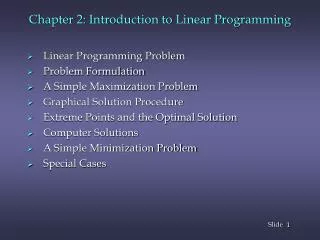
Chapter 2: Linear Programming. Dr. Alaa Sagheer 2010-2011. Chapter Outline. Part I:. Introduction The Linear Programming Model Examples of Linear Programming Problems Developing Linear Programming Models Graphical Solution to LP Problems. Introduction.

E N D
Chapter 2: Linear Programming Dr. Alaa Sagheer 2010-2011
Chapter Outline Part I: • Introduction • The Linear Programming Model • Examples of Linear Programming Problems • Developing Linear Programming Models • Graphical Solution to LP Problems
Introduction • Mathematical programming is used to find the best or optimal solution to a problem that requires a decision or set of decisions about how best to use a set of limited resources to achieve a state goal of objectives. • Steps involved in mathematical programming • Conversion of stated problem into a mathematical model that abstracts all the essential elements of the problem. • Exploration of different solutions of the problem. • Finding out the most suitable or optimum solution. • Linear programming requires that all the mathematical functions in the model be linear functions.
Introduction Example: The Burroughs garment company manufactures men's shirts and women’s blouses for Walmark Discount stores. Walmark will accept all the production supplied by Burroughs. The production process includes cutting, sewing and packaging. Burroughs employs 25 workers in the cutting department, 35 in the sewing department and 5 in the packaging department. The factory works one 8-hour shift, 5 days a week. The following table gives the time requirements and the profits per unit for the two garments:
Introduction Minutes per unit Determine the optimal weekly production schedule for Burroughs.
Introduction Solution:Assume that Burroughs produces x1 shirts and x2 blouses per week: Profit got = 8 x1 + 12 x2 Time spent on cutting = 20 x1 + 60 x2 mts Time spent on sewing = 70 x1 + 60 x2 mts Time spent on packaging = 12 x1 + 4 x2 mts
Introduction The objective is to find x1, x2 so as to maximize the profit z = 8 x1 + 12 x2 satisfying the constraints: 20 x1 + 60 x2≤ 25 40 60 70 x1 + 60 x2 ≤ 35 40 60 12 x1 + 4 x2 ≤ 5 40 60 x1, x2≥ 0, integers
Introduction This is a typical optimization problem Any values of x1, x2 that satisfy all the constraints of the model is called a feasible solution. We are interested in finding the optimum feasible solution that gives the maximum profit while satisfying all the constraints.
The Linear Programming Model Let x1, x2, x3, ………, xn are decision variables and Z = Objective function or linear function Requirement: Maximization of the linear function Z Z = c1x1 + c2x2 + c3x3 + ………+ cnxn subject to the following constraints: where aij, bi, and cj are given constants.
The Linear Programming Model • The linear programming model can be written in more efficient notation as: The decision variables, xI, x2, ..., xn, represent levels of ncompeting activities
The Linear Programming Model An LPP satisfies the three basic properties: 1. Proportionality: It means, the contributions of each decision variable in the objective function and its requirements in the constraints are directly proportional to the value of the variable 2. Additivity: This property requires the contribution of all the variables in the objective function and its constraints to be the direct sum of individual contributions of each variables. 3. Certainty: All the objective and constraint coefficient of the LP model are deterministic. This mean that they are known constants- a rare occurrence in real life.
Examples of LP Problems 1. A Product Mix Problem • A manufacturer has fixed amounts of different resources such as raw material, labor, and equipment. • These resources can be combined to produce any one of several different products. • The quantity of the ith resource required to produce one unit of the jthproduct is known. • The decision maker wishes to produce the combination of products that will maximize total income.
Examples of LP Problems 2. A Blending Problem • Blending problems refer to situations in which a number of components (or commodities) are mixed together to yield one or more products. • Typically, different commodities are to be purchased. Each commodity has known characteristics and costs. • The problem is to determine how much of each commodity should be purchased and blended with the rest so that the characteristics of the mixture lie within specified bounds and the total cost is minimized.
Examples of LP Problems 3. A Production Scheduling Problem • A manufacturer knows that he must supply a given number of items of a certain product each month for the next n months. • They can be produced either in regular time, subject to a maximum each month, or in overtime. The cost of producing an item during overtime is greater than during regular time. A storage cost is associated with each item not sold at the end of the month. • The problem is to determine the production schedule that minimizes the sum of production and storage costs.
Examples of LP Problems 4. A Transportation Problem • A product is to be shipped in the amounts al, a2, ..., amfrom m shipping origins and received in amounts bl, b2, ..., bnat each of n shipping destinations. • The cost of shipping a unit from the ith origin to the jthdestination is known for all combinations of origins and destinations. • The problem is to determine the amount to be shipped from each origin to each destination such that the total cost of transportation is a minimum.
Examples of LP Problems 5. A Flow Capacity Problem • One or more commodities (e.g., traffic, water, information, cash, etc.) are flowing from one point to another through a network whose branches have various constraints and flow capacities. • The direction of flow in each branch and the capacity of each branch are known. • The problem is to determine the maximum flow, or capacity of the network.
Developing LP Model • The variety of situations to which linear programming has been applied ranges from agriculture to zinc melting. • Steps Involved: • Determine the objective of the problem and describe it by a criterion function in terms of the decision variables. • Find out the constraints. • Do the analysis which should lead to the selection of values for the decision variables that optimize the criterion function while satisfying all the constraints imposed on the problem.
Developing LP Model Graphical Solution + Example: Product Mix Problem The N. Dustrious Company produces two products: I and II. The raw material requirements, space needed for storage, production rates, and selling prices for these products are given in Table I. The total amount of raw material available per day for both products is 15751b. The total storage space for all products is 1500 ft2, and a maximum of 7 hours per day can be used for production.
Developing LP Model Example: Product Mix Problem All products manufactured are shipped out of the storage area at the end of the day. Therefore, the two products must share the total raw material, storage space, and production time. The company wants to determine how many units of each product to produce per day to maximize its total income Solution • The company has decided that it wants to maximize its sale income, which depends on the number of units of product I and II that it produces. • Therefore, the decision variables, x1 and x2can be the number of units of products I and II, respectively, produced per day.
Developing LP Model • The object is to maximize the equation: • Z = 13x1 + 11x2 • subject to the constraints on storage space, raw materials, and production time. • Each unit of product I requires 4 ft2 of storage space and each unit of product II requires 5 ft2. Thus a total of 4x1 + 5x2 ft2 of storage space is needed each day. This space must be less than or equal to the available storage space, which is 1500 ft2. Therefore, • 4X1 + 5X2 1500 • Similarly, each unit of product I and II produced requires 5 and 3 1bs, respectively, of raw material. Hence a total of 5xl + 3x2Ib of raw material is used.
Developing LP Model • This must be less than or equal to the total amount of raw material available, which is 1575 Ib. Therefore, • 5x1 + 3x2 1575 • Prouct I can be produced at the rate of 60 units per hour. Therefore, it must take I minute or 1/60 of an hour to produce I unit. Similarly, it requires 1/30 of an hour to produce 1 unit of product II. Hence a total of x1/60 + x2/30 hours is required for the daily production. This quantity must be less than or equal to the total production time available each day. Therefore, • x1 / 60 + x2 / 30 7 • or x1 + 2x2 420 • Finally, the company cannot produce a negative quantity of any product, therefore x1 and x2must each be greater than or equal to zero.
Developing LP Model Graphical Solution • The linear programming model for this example can be summarized as:
Developing LP Model Graphical Solution +Example (2): Reddy Mikks produce both interior and exterior paints from two raw materials, M1 and M2. The following table provides the basic data of the problem:
Developing LP Model Example Problem A market survey indicates that the daily demand for the interior paint cannot exceed that for extirior paint by more than one ton. Also, the maximam daily demand for the interior paint is 2 tons. Reddy Mikks wants to determine the optimum(best) product mix of the interior and exterior paints that maximizes the total daily profit. Solution • Reddy Mikks has decided that it wants to maximize its total daily profit, which depends on the product mix of the interior and exterior paints. • Therefore, the decision variables, x1 and x2can be the ton of exterior and interior paints, respectively, produced per day.
Developing LP Model • The object is to maximize the equation: • Z = 5x1 + 4x2 • The daily raw material M1 is 6tons per ton of exterior paint and 4 tons per ton of interior paint must be equal the daily avaliability of raw material M1 (24 ton) , Therefore, • 6x1+ 4x2 24 • Similary, The daily usage of raw material M2 is 1ton per ton of exterior paint and 2 tons per ton of interior paint must be equal the daily aviliability or raw material M2 (6 tons), Therefore, • x1+ 2x2 6
Developing LP Model • The first demand restriction stipulates that the excess the daily production of interior over exterior paint should not exceed 1 ton, Therefore , • x2 - x1 1 • The second demand restrection stipulates that the maximum daily demand of interior paint is limited to 2 tons. Therefore, • x2 2
Developing LP Model Graphical Solution • The linear programming model for this example can be summarized as:
Developing LP Model Example (3): Wild West produces two types of cowboy hats. Type I hat requires twice as much labor as a Type II. If all the available labor time is dedicated to Type II alone, the company can produce a total of 400 Type II hats a day. The respective market limits for the two types of hats are 150 and 200 hats per day. The profit is $8 per Type I hat and $5 per Type II hat. Formulate the problem as an LPP so as to maximize the profit.
Developing LP Model Solution: Assume that Wild West produces x1 Type I hats and x2 Type II hats per day. 8 x1 + 5 x2 Per day Profit got = Assume the time spent in producing one type II hat is c minutes. Labour Time spent is (2 x1 + x2) c minutes
Developing LP Model The objective is to find x1, x2 so as to maximize the profit z = 8 x1 + 5 x2 satisfying the constraints: (2 x1 + x2 ) c ≤ 400 c x1 ≤ 150 x2 ≤ 200 x1, x2≥ 0, integers
Developing LP Model Example (4): BITS wants to host a Seminar for five days. For the delegates there is an arrangement of dinner every day. The requirement of napkins during the 5 days is as follows:
Developing LP Model Institute does not have any napkins in the beginning. After 5 days, the Institute has no more use of napkins. A new napkin costs Rs. 2.00. The washing charges for a used one are Rs. 0.50. A napkin given for washing after dinner is returned the third day before dinner. The Institute decides to accumulate the used napkins and send them for washing just in time to be used when they return. How shall the Institute meet the requirements so that the total cost is minimized ? Formulate as a LPP.
Developing LP Model Solution: Let xj be the number of napkins purchased on day j, j=1,2,..,5 Let yj be the number of napkins given for washing after dinner on day j, j=1,2,3 Thus we must have x1 = 80, x2 = 50, x3 + y1 = 100, x4 + y2 = 80 x5 + y3 = 150 Also we have y1 ≤ 80, y2 ≤ (80 – y1) + 50 y3 ≤ (80 – y1) + (50 – y2) + 100
Developing LP Model Thus we have to Minimize z = 2(x1+x2+x3+x4+x5)+0.5(y1+y2+y3) Subject to x1 = 80, x2 = 50, x3 +y1 =100, x4 + y2 = 80, x5 + y3 = 150, y1≤ 80, y1+y2 ≤ 130, y1+y2+y3≤ 230, all variables ≥ 0, integers
Developing LP Model Example (5): A Post Office requires different number of full-time employees on different days of the week. The number of employees required on each day is given in the table below. Union rules say that each full-time employee must receive two days off after working for five consecutive days. The Post Office wants to meet its requirements using only full-time employees. Formulate the above problem as a LPP so as to minimize the number of full-time employees hired.
Developing LP Model Requirements of full-time employees day-wise
Developing LP Model Solution: Let xi be the number of full-time employees employed at the beginning of day i (i = 1, 2, …, 7). Thus our problem is to find xiso as to Minimize Subject to
The Graphical Solution • The determination of the solution space that defines the feasible solutions that satisfy all the constrains of the model. • The determination of the optimum solution from among all the points in the feasible solution space.
Graphical LP Solution Model Example: Electra produces two types of electric motors, each on a separate assembly line. The respective daily capacities of the two lines are 150 and 200 motors. Type I motor uses 2 units of a certain electronic component, and type II motor uses only 1 unit. The supplier of the component can provide 400 pieces a day.The profits per motor of types I and II are $8 and $5 respectively. Formulate the problem as a LPP and find the optimal daily production.
Graphical LP Solution Model Let the company produce x1 type I motors and x2 type II motors per day. The objective is to find x1 and x2 so as to Maximize the profit Subject to the constraints
Graphical LP Solution Model Step 1 Determination of the Feasible solution space The non-negativity restrictions tell that the solution space is in the first quadrant. Then we replace each inequality constraint by an equality and then graph the resulting line (noting that two points will determine a line uniquely). Step 2 Determination of the optimal solution The determination of the optimal solution requires the direction in which the objective function will increase (decrease) in the case of a maximization (minimization) problem. We find this by assigning two increasing (decreasing) values for z and then drawing the graphs of the objective function for these two values. The optimum solution occurs at a point beyond which any further increase (decrease) of z will make us leave the feasible space.
Graphical solution x2 Maximize z=8x1+5x2 Subject to the constraints Optimum =1800 at 2x1+x2 400 x1 150 x2 200 x1,x2 0 (100,200) (0,200) z=1200 (150,100) z=1800 z=1000 x1 z=400 (150,0) z=1700
Graphical LP Solution Model Realted to Reddy Mikks problem Problem
Graphical Solution to LP Problems Related to Product Mix Problem Problem
Graphical LP Solution Model Feed Mix Problem Minimize z = 2x1 + 3x2 Subject to x1 + 3 x2 15 2 x1 + 2 x2 20 3 x1 + 2 x2 24 x1, x2 0
Graphical Solution of Feed Mix Problem (0,12) z = 26 z = 30 z= 36 z = 39 (4,6) z = 42 z = 22.5 Minimum at (7.5,2.5) (15,0)
Graphical LP Solution Model (5) Maximize z = 2x1 + x2 Subject to x1 + x2≤ 40 4 x1 + x2 ≤ 100 x1, x2≥ 0 Optimum = 60 at (20, 20)
Graphical solution (0,40) z maximum at (20,20) (25,0)
The Graphical Solution Graphical Solution Ozark farms uses at least 800 Ib of special feed is a mixture of corn and soybean meal with the following compositions: The dietary requirement of the special feed are at least 30% protein and at most 5% fiber. Ozark Farms wishes to determine the daily minimm- cost feed mix.
The Graphical Solution Graphical Solution Solution We can consider that, And the objective function seeks to minimize the total daily cost (in dollars) of the feed mix and is thus expressed as Subject to constrains: