More details can be found in the “ Course Objectives and Content ” handout on the course webpage.

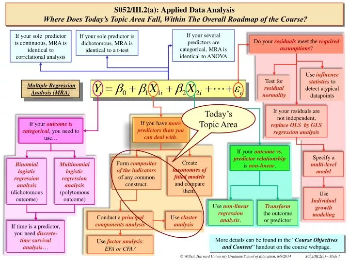
1. If your several predictors are categorical, MRA is identical to ANOVA If your sole predictor is continuous, MRA is identical to correlational analysis If your sole predictor is dichotomous, MRA is identical to a t-test Do your residuals meet the requiredassumptions? Use influence statistics to detect atypical datapoints Test for residual normality Multiple Regression Analysis (MRA) If your residuals are not independent, replace OLS byGLS regression analysis If you have more predictors than you can deal with, Today’s Topic Area If your outcome is categorical, you need to use… If your outcome vs. predictor relationship isnon-linear, Specify amulti-level model Create taxonomies of fitted models and compare them. Form composites of the indicators of any common construct. Binomiallogistic regression analysis (dichotomous outcome) Multinomial logistic regression analysis (polytomous outcome) Use Individual growth modeling Use non-linear regression analysis. Transform the outcome or predictor Conduct a principal components analysis Use cluster analysis If time is a predictor, you need discrete-time survival analysis… More details can be found in the “Course Objectives and Content” handout on the course webpage. S052/III.2(a):Applied Data AnalysisWhere Does Today’s Topic Area Fall, Within The Overall Roadmap of the Course? Use factor analysis: EFA or CFA?

2. S052/III.2(a): Exploratory Cluster Analysis of VariablesHow Does Today’s Topic Map Onto The Printed Syllabus? Please check inter-connections among the Roadmap, the Daily Topic Area, the Printed Syllabus, and the content of today’s class when you pre-read the day’s materials. Taking a Different Perspective on the Standard PCA Solution (Slides 4-11). The Cluster Analysis of Variables (Slide 13-20). Which Strategy For Forming Composites Of Multiple Indicators Is The “Best”? (Slide 22).

3. S052/III.2(a): Exploratory Cluster Analysis of VariablesHow Does Today’s Topic Map Onto The Printed Syllabus? • Taking a Different Perspective on the Standard PCA Solution (Slides 4-11). Please check inter-connections among the Roadmap, the Daily Topic Area, the Printed Syllabus, and the content of today’s class when you pre-read the day’s materials.

4. S052/III.2(a): Exploratory Cluster Analysis of VariablesTaking a Different Perspective on the Standard PCA Solution • Here’s a dataset in which teachers’ responses to what the investigators believed were multiple indicators of a single underlying construct of Teacher Job Satisfaction: • The data described in TSUCCESS_info.pdf. Principal Component and Frau Himmler

5. Looking for the scree? S052/III.2(a): Exploratory Cluster Analysis of VariablesTaking a Different Perspective on the Standard PCA Solution Recall our earlier scree plot inspection of the eigenvalues from the teacher satisfaction example…. Eigenvalues of the Correlation Matrix Eigenvalue Difference Proportion Cumulative 1 2.60599489 1.39439026 0.4343 0.4343 2 1.21160463 0.49880170 0.2019 0.6363 3 0.71280293 0.11761825 0.1188 0.7551 4 0.59518468 0.14741881 0.0992 0.8543 5 0.44776587 0.02111886 0.0746 0.9289 6 0.42664701 0.0711 1.0000 We concluded that this scree plot suggested there may be two important dimensionsof information being measured by the six indicators as a group.

6. Previously, we’ve interpreted the elements of these eigenvectors as representing how each of the six original (standardized) indicators is weighted in the orthogonal compositevariables PC_1 & PC_2. • Each indicator loads on PC_1 & PC_2 in different ways and, by inspecting the magnitude and direction of the loadings, we have concluded that PC_1 & PC_2 measure: • TeacherEnthusiasm, and • TeacherFrustration, respectively. • But now, let’s adopt a different perspective: • Rather than trying to interpret PC_1 and PC_2 separately as composite variables that measure uncorrelated features of teacher job satisfaction, • Let’s regard PC_1 and PC_2 as defining orthogonal directions in an underlying two-dimensional space, in which the six original indicators can now be plotted efficiently : • Let’s try to imagine what the six original variables “look like” in that reduced space. S052/III.2(a): Exploratory Cluster Analysis of VariablesTaking a Different Perspective on the Standard PCA Solution This suggests that the 1stand 2nd eigenvectors are most interesting, and that perhaps we can ignore the rest … Principal components (eigenvectors) ------------------------------------------------------------------------ Variable | Comp1 Comp2 Comp3 Comp4 Comp5 Comp6 ----------+------------------------------------------------------------ X1 | 0.3472 0.6182 0.0896 0.0264 0.6261 0.3108 X2 | 0.3617 0.5950 0.0543 -0.0217 -0.6685 -0.2548 X3 | 0.3778 -0.3021 0.7555 0.4028 0.0503 -0.1746 X4 | 0.4144 -0.1807 -0.5972 0.6510 -0.0493 0.1129 X5 | 0.4727 -0.2067 -0.2418 -0.4501 0.3022 -0.6176 X6 | 0.4591 -0.3117 0.0558 -0.4584 -0.2548 0.6433 ------------------------------------------------------------------------

7. Loadings on Comp1 0.8 0.6 0.4 0.2 0 -0.8 -0.6 -0.4 -0.2 0 0.2 0.4 0.6 0.8 Loadings on Comp2 S052/III.2(a): Exploratory Cluster Analysis of VariablesTaking a Different Perspective on the Standard PCA Solution This is easiest to imagine by plotting the elements of the eigenvectors on the same plot, as follows ... Eigenvectors Comp1Comp2 X1 Have high standards of teaching 0.3472 0.6182 X2 Continually learning on job 0.3617 0.5950 X3 Successful in educating students 0.3778 -.3021 X4 Waste of time to do best as teacher 0.4144 -.1807 X5 Look forward to working at school 0.4727 -.2067 X6 Time satisfied with job 0.4591 -.3117

8. First Pass, to provide the initial principal components analysis of all six indicators. S052/III.2(a): Exploratory Cluster Analysis of VariablesAn Example of The Cluster Analysis of Variables Here’s the STATAcode for Handout III.2(a).1, in which I regroup the indicators and composite them within sensible groups … <Usual data-input statements omitted> … *------------------------------------------------------------------------------ * Carry-out the principal components analysis interactively, in successively * smaller groups of variables, selected based on the prior pca. *------------------------------------------------------------------------------ * First pca of all the indicators, to determine the initial structure: pca X1-X6, means * Second pass, within groups of indicators established in the first pass: * Group #1, output scores on the first component in the group: pca X1 X2, means predict GP1_PC1 * Group #2, output scores on the first component in the group: pca X3 X4 X5 X6, means predict GP2_PC1 *------------------------------------------------------------------------------ * Inspect the properties of composite scores obtained. *------------------------------------------------------------------------------ * List out the indicator and principal component scores for first 35 teachers: list X1-X6 GP1_PC1 GP2_PC1 in 1/35, nolabel * Estimate univariate descriptive statistics for the two composite scores: tabstat GP1_PC1 GP2_PC1, stat(n mean sd) columns(statistics) * Estimate the bivariate correlation between the two composite scores on: pwcorr GP1_PC1 GP2_PC1, sig obs Second Passto composite indicators in Group #1, consisting of variables X1 & X2, and provide composites with prefix GP1_ . Hopefully, a single composite will capture most of the variation in X1 & X2. Second Passto composite indicators in Group #2, consisting of variables X3, X4, X5 & X6, and provide composites with prefix GP2_ . Hopefully, a single composite will again capture most of the important variation in X3, X4, X5 & X6. • Inspect the statistical properties of the obtained “sub-group” composites: • List out the values of a few cases. • Obtain univariate descriptive statistics on each composite. • Estimate the bivariate correlation between of the composites.

9. Successful first principal component of X1 & X2, containing almost 78% of the initial two units of standardized variance. • Teachers who score high on this composite… • Have high standards of teaching performance. • Feel that they are continually learning on the job. A composite measure ofTEACHER PERFORMANCE? S052/III.2(a): Exploratory Cluster Analysis of VariablesAn Example of The Cluster Analysis of Variables Here’s the PCA output for theprincipal components analysis of the first group of indicators (X1 & X2) … Principal components/correlation Number of obs = 5058 Number of comp. = 2 Trace = 2 Rotation: (unrotated = principal) Rho = 1.0000 -------------------------------------------------------------------------- Component | Eigenvalue Difference Proportion Cumulative -------------+------------------------------------------------------------ Comp1 | 1.55199 1.10397 0.7760 0.7760 Comp2 | .448013 . 0.2240 1.0000 -------------------------------------------------------------------------- Principal components (eigenvectors) ----------------------------------- Variable | Comp1 Comp2 -------------+--------------------- X1 | 0.7071 0.7071 X2 | 0.7071 -0.7071 -----------------------------------

10. Successful first principal component of X3, X4, X5 & X6, containing 56% of the initial four units of standardized variance. • Teachers who score high on this composite… • Believe they are successful in educating students. • Feel that it is not a waste of time to be a teacher. • Look forward to working at school. • Are always satisfied on the job A composite measure of TEACHER FEELINGS? S052/III.2(a): Exploratory Cluster Analysis of VariablesAn Example of The Cluster Analysis of Variables Here’s the PCA output for theprincipal components analysis of the second group of indicators (X3 thru X6) … Principal components/correlation Number of obs = 5031 Number of comp. = 4 Trace = 4 Rotation: (unrotated = principal) Rho = 1.0000 -------------------------------------------------------------------------- Component | Eigenvalue Difference Proportion Cumulative -------------+------------------------------------------------------------ Comp1 | 2.25102 1.52944 0.5628 0.5628 Comp2 | .721572 .127624 0.1804 0.7431 Comp3 | .593948 .160484 0.1485 0.8916 Comp4 | .433464 . 0.1084 1.0000 -------------------------------------------------------------------------- Principal components (eigenvectors) ------------------------------------------------------- Variable | Comp1 Comp2 Comp3 Comp4 -------------+----------------------------------------- X3 | 0.4509 0.7636 0.4248 0.1820 X4 | 0.4687 -0.5960 0.6358 -0.1447 X5 | 0.5344 -0.2260 -0.4516 0.6778 X6 | 0.5398 0.1033 -0.4599 -0.6975 -------------------------------------------------------

11. S052/III.2(a): Exploratory Cluster Analysis of VariablesAn Example of The Cluster Analysis of Variables +-----------------------------------------------+ | X1 X2 X3 X4 X5 X6 GP1_PC1 GP2_PC1 | |-----------------------------------------------| | 5 5 3 3 4 2 1.074 -1.404 | | 4 3 2 1 1 2 -0.711 -3.842 | | 4 4 2 2 2 2 -0.143 -3.159 | | . 6 3 5 3 3 . -0.299 | | 4 4 3 2 4 3 -0.143 -0.740 | |-----------------------------------------------| | . 5 2 4 3 3 . -1.251 | | 4 4 4 4 5 3 -0.143 0.894 | | 6 4 4 1 1 2 1.154 -2.500 | | 6 6 3 6 5 3 2.291 0.785 | | 3 5 3 6 3 3 -0.223 -0.018 | |-----------------------------------------------| | 4 2 1 3 2 2 -1.279 -3.550 | | 5 6 2 6 6 4 1.642 1.460 | | 4 3 3 2 5 3 -0.711 -0.339 | | 3 3 3 3 4 3 -1.360 -0.459 | | 4 4 3 6 3 2 -0.143 -0.963 | … variable | N mean sd ----------+--------------------- GP1_PC1 | 5058 0 1.246 GP2_PC1 | 5031 0 1.500 -------------------------------- • Everyone with complete data has a 1st component score on each new grouping of indicators, • But, because they were obtained in separate PCAs, the two composite scores are no longer uncorrelated with each other. | GP1_PC1 GP2_PC1 -------------+------------------ GP1_PC1 | 1.0000 | 5058 | GP2_PC1 | 0.3245 1.0000 | 4955 5031

12. S052/III.2(a): Exploratory Cluster Analysis of VariablesHow Does Today’s Topic Map Onto The Printed Syllabus? Please check inter-connections among the Roadmap, the Daily Topic Area, the Printed Syllabus, and the content of today’s class when you pre-read the day’s materials. The Cluster Analysis of Variables (Slide 13-20).

13. Before you can use the “cva” routine, you must download it, into your version of STATA, because it is a user-supported routine. Additional instructions are provided in the comments of the Data-Analytic Handout itself. Calls on cvato cluster indicators X1 through X6. The cva routine works by conducting multiple PCA’s, so we can gain insight into its functioning by conducting a few ourselves. Got to ensure listwise deletion of cases with missing data first, to ensure comparability of output. These are the PCA’s that correspond to the decision steps in the clv analysis. S052/III.2(a): Exploratory Cluster Analysis of Variables An Example of The Cluster Analysis of Variables There’s a routine in STATA that conducts a similar clustering of variables automatically. It’s called “clv”… and its use is featured in Data-Analytic Handout III.2(a).2 … < usual data-input statements have been omitted … > • *-------------------------------------------------------------------------------- • * Conducting a cluster analysis of variables. • *-------------------------------------------------------------------------------- • * Before you execute the rest of this code, make sure the STATA user-supported • * routine "clv" is available on your workstation. Check by typing "help clv." • *  • * Now, perform a cluster analysis of all six indicators of teacher satisfaction: • clv X1 X2 X3 X4 X5 X6, textsize(small) • *-------------------------------------------------------------------------------- • * Some important ancillary PCA analyses • *-------------------------------------------------------------------------------- • * To gain insight into the "clv" clustering process, it's useful to conduct some • * selected ancillary pca analyses, which mirror the critical steps in the "clv" • * algorithm itself. • * First, we must conduct a listwise deletion of cases with missing values to • * ensure that the sample for the ancillary analyses is identical to that used in • * the clv application, as follows: • dropmiss, obs any • * The following steps mirror the steps of the clv process. however, the clv • * routine carries out far more subsidiary PCA analyses than are listed below, • * in order to make its critical clustering decisions. But, these steps are the • * critical decision steps whose consequences appear as summary statistics in the • * clv output that you will obtain above. • * Step #1: Combine X1 and X2 to form Object#7: • pca X1 X2 • * Step #2: Combine X5 and X6 to form Object#8: • pca X5 X6 • * Step #3: Combine X4 and Object#8(X5,X6) to form Object#9: • pca X4 X5 X6 • * Step #4: Combine X3 and Object#9(X4,(X5,X6)) to form Object#10: • pca X3 X4 X5 X6 • * Step #5: Combine Object#7(X1,X2) and Object#10(X3,(X4,(X5,X6))) to form Object#11: • pca X1 X2 X3 X4 X5 X6

14. S052/III.2(a): Exploratory Cluster Analysis of VariablesAn Example of The Cluster Analysis of Variables The cluster solution is easier to comprehend if it is plotted as a tree diagramor dendrogram: X1 X2 X3 X4 X5 X6 The vertical axis displays the percentage of the total standardized variance in the original indicators that is notcontained in the composites have been formed, at this level of clustering … as follows:

15. S052/III.2(a): Exploratory Cluster Analysis of VariablesAn Example of The Cluster Analysis of Variables Here’s the clustering process: -------------------------------- TOTAL VARIANCE: 6.00000 NUMBER OF INDIVIDUALS: 4955 METHOD: CLASSICAL -------------------------------- ----------------------------------------------------------------------- # of T Explained Step clusters Child 1 Child 2 Parent T value Variance ----------------------------------------------------------------------- 1 5 X1 X2 7 5.5548 92.581% 2 4 X5 X6 8 5.1077 85.128% 3 3 X4 8 9 4.4912 74.853% 4 2 X3 9 10 3.8086 63.477% 5 1 7 10 11 2.6060 43.433% ----------------------------------------------------------------------- • Before the Clustering begins… • There are 6 original “Objects “: • Indicators X1 thru X6: • Referred to, oddly, as “children.” • Each contributes one unit of original standardized variability to the compositing process. • Thus, the total sum of original standardized variance: • T = 1 + 1 + 1 + 1 + 1 + 1 = 6 • First Step… • PCA is conducted on each of all-possible pairs of objects: • Value of first eigenvalue is noted, in each analysis. • That pairof objects which can be combined best are identified: • Here, objects X1 & X2 have largest first eigenvalue of any pair of objects, at this step (1.5548), • They are then joined and treated as a single object from here on, named Object #7 (see “Parent” column). • There are now five objects remaining: • Original ObjectsX3, X4, X5 & X6, and • Newly formed Object #7, a cluster of X1 & X2. • Total variability in remaining objects is now: • T = 1.5548 + 1+ 1+ 1 + 1 = 5.5548 units (or 92.58% of 6). PCA of X1 & X2 Rotation: (unrotated = principal) ----------------------------------------- Component | Eigenvalue Difference -------------+--------------------------- Comp1 | 1.55484 1.10968 Comp2 | .445159 . ----------------------------------------- Eigenvectors ---------------------------------- Variable | Comp1 Comp2 -------------+-------------------- X1 | 0.7071 0.7071 X2 | 0.7071 -0.7071 ----------------------------------

16. S052/III.2(a): Exploratory Cluster Analysis of VariablesAn Example of The Cluster Analysis of Variables Here’s the clustering process: -------------------------------- TOTAL VARIANCE: 6.00000 NUMBER OF INDIVIDUALS: 4955 METHOD: CLASSICAL -------------------------------- ----------------------------------------------------------------------- # of T Explained Step clusters Child 1 Child 2 Parent T value Variance ----------------------------------------------------------------------- 1 5 X1 X2 7 5.5548 92.581% 2 4 X5 X6 8 5.1077 85.128% 3 3 X4 8 9 4.4912 74.853% 4 2 X3 9 10 3.8086 63.477% 5 1 7 10 11 2.6060 43.433% ----------------------------------------------------------------------- • Second Step… • PCA is conducted on each of all-possible remaining pairs of objects: • Value of first eigenvalue is noted, in each analysis. • That pairof objects which can be combined best are identified: • Here, objects X5 & X6 have largest first eigenvalue of any pair of objects, at this step (1.5529), • They are then joined and treated as a single object from here on, named Object #8 (see “Parent” column). • There are now four objects remaining: • Original ObjectsX3 & X4, and • Object #7 & newly formed Object #8, a cluster of X5 & X6. • Total variability in remaining objects is now: • T = 1.5548 + 1 + 1+ 1.5529 = 5.1077 units (or 85.13% of 6). • PCA of X5 & X6 Rotation: (unrotated = principal) ----------------------------------------- Component | Eigenvalue Difference -------------+--------------------------- Comp1 | 1.55286 1.10573 Comp2 | .447136 . ------------------------------------------ • Eigenvectors ---------------------------------- Variable | Comp1 Comp2 -------------+-------------------- X5 | 0.7071 0.7071 X6 | 0.7071 -0.7071 ----------------------------------

17. S052/III.2(a): Exploratory Cluster Analysis of VariablesAn Example of The Cluster Analysis of Variables Here’s the clustering process: -------------------------------- TOTAL VARIANCE: 6.00000 NUMBER OF INDIVIDUALS: 4955 METHOD: CLASSICAL -------------------------------- ----------------------------------------------------------------------- # of T Explained Step clusters Child 1 Child 2 Parent T value Variance ----------------------------------------------------------------------- 1 5 X1 X2 7 5.5548 92.581% 2 4 X5 X6 8 5.1077 85.128% 3 3 X4 8 9 4.4912 74.853% 4 2 X3 9 10 3.8086 63.477% 5 1 7 10 11 2.6060 43.433% ----------------------------------------------------------------------- • Third Step… • PCA is conducted on each of all-possible remaining pairs of objects: • Value of first eigenvalue is noted, in each analysis. • That pairof objects which can be combined best are identified: • Here, X4 & Object #8 have largest first eigenvalue of any pair of objects, at this step (1.9364), • They are then joined and treated as a single object from here on, named Object #9 (see “Parent” column). • There are now three objects remaining: • Original Object X3, and • Object #7 & newly formed Object #9, a cluster of X4,X5 & X6. • Total variability in remaining objects is now: • T = 1.5548 + 1 + 1.9364 = 4.4912 units (or 74.85% of 6). • PCA of X4, X5 & X6 Rotation: (unrotated = principal) ----------------------------------------- Component | Eigenvalue Difference -------------+--------------------------- Comp1 | 1.93635 1.31481 Comp2 | .621538 .179423 Comp3 | .442115 . ----------------------------------------- • Eigenvectors ---------------------------------- Variable | Comp1 Comp2 -------------+-------------------- X4 | 0.5392 0.8298 X5 | 0.6043 -0.2618 X6 | 0.5867 -0.4929 ----------------------------------

18. S052/III.2(a): Exploratory Cluster Analysis of VariablesAn Example of The Cluster Analysis of Variables Here’s the clustering process: -------------------------------- TOTAL VARIANCE: 6.00000 NUMBER OF INDIVIDUALS: 4955 METHOD: CLASSICAL -------------------------------- ----------------------------------------------------------------------- # of T Explained Step clusters Child 1 Child 2 Parent T value Variance ----------------------------------------------------------------------- 1 5 X1 X2 7 5.5548 92.581% 2 4 X5 X6 8 5.1077 85.128% 3 3 X4 8 9 4.4912 74.853% 4 2 X3 9 10 3.8086 63.477% 5 1 7 10 11 2.6060 43.433% ----------------------------------------------------------------------- • Fourth Step… • PCA is conducted on each of all-possible remaining pairs of objects: • Value of first eigenvalue is noted, in each analysis. • That pairof objects which can be combined best are identified: • Here, X3 & Object #9 have largest first eigenvalue of any pair of objects, at this step (2.2538), • They are then joined and treated as a single object from here on, named Object #10 (see “Parent” column). • There are now two objects remaining: • Object #7 & newly formed Object #10, a cluster of X3, X4,X5 & X6. • Total variability in remaining objects is now: • T = 1.5548 + 2.2538= 3.8086 units (or 63.48% of 6). • PCA of X3, X4, X5, X6 Rotation: (unrotated = principal) ----------------------------------------- Component | Eigenvalue Difference -------------+--------------------------- Comp1 | 2.25375 1.53467 Comp2 | .719086 .124064 Comp3 | .595022 .162881 Comp4 | .432141 . ----------------------------------------- • Eigenvectors • ---------------------------------- Variable | Comp1 Comp2 -------------+-------------------- X3 | 0.4499 0.7759 X4 | 0.4700 -0.5791 X5 | 0.5337 -0.2340 X6 | 0.5402 0.0889 ----------------------------------

19. S052/III.2(a): Exploratory Cluster Analysis of VariablesAn Example of The Cluster Analysis of Variables Here’s the clustering process: -------------------------------- TOTAL VARIANCE: 6.00000 NUMBER OF INDIVIDUALS: 4955 METHOD: CLASSICAL -------------------------------- ----------------------------------------------------------------------- # of T Explained Step clusters Child 1 Child 2 Parent T value Variance ----------------------------------------------------------------------- 1 5 X1 X2 7 5.5548 92.581% 2 4 X5 X6 8 5.1077 85.128% 3 3 X4 8 9 4.4912 74.853% 4 2 X3 9 10 3.8086 63.477% 5 1 7 10 11 2.6060 43.433% ----------------------------------------------------------------------- • PCA of X1, X2, X3, X4, X5 & X6 Rotation: (unrotated = principal) ----------------------------------------- Component | Eigenvalue Difference -------------+--------------------------- Comp1 | 2.60599 1.39439 Comp2 | 1.2116 .498802 Comp3 | .712803 .117618 Comp4 | .595185 .147419 Comp5 | .447766 .0211189 Comp6 | .426647 . ----------------------------------------- • Eigenvectors ---------------------------------- Variable | Comp1 Comp2 -------------+-------------------- X1 | 0.3472 0.6182 X2 | 0.3617 0.5950 X3 | 0.3778 -0.3021 X4 | 0.4144 -0.1807 X5 | 0.4727 -0.2067 X6 | 0.4591 -0.3117 ---------------------------------- • Fifth Step… • PCA is conducted on each of all-possible remaining pairs of objects: • Value of first eigenvalue is noted, in each analysis. • That pairof objects which can be combined best are identified: • Here, Object #7 & Object #10 have largest first eigenvalue of any pair of objects, at this step (2.6060), • They are then joined and treated as a single object from here on, named Object #11 (see “Parent” column). • There is now one object remaining: • Newlyformed Object #11, a cluster of X1, X2, X3, X4,X5 & X6. • Total variability in remaining objects is now: • T = 2.6060 = 2.6060 units (or 43.43% of 6).

20. S052/III.2(a): Exploratory Cluster Analysis of VariablesAn Example of The Cluster Analysis of Variables -------------------------------------------------------------- # of T Explained Step clusters Child 1 Child 2 Parent T value Variance -------------------------------------------------------------- 1 5 X1 X2 7 5.5548 92.581% 2 4 X5 X6 8 5.1077 85.128% 3 3 X4 8 9 4.4912 74.853% 4 2 X3 9 10 3.8086 63.477% 5 1 7 10 11 2.6060 43.433% -------------------------------------------------------------- Tying it all together … X1 X2 X3 X4 X5 X6 100% - 85.13% = 14.87% 100% - 43.43% = 54.57% 100% - 74.85% = 25.15% 100% - 63.48% = 36.42% 100% - 92.58% = 7.42% Vertical axis displays the percentage of the total standardized variance in the original indicators that is notcontained in the composites formed at this level of clustering.

21. S052/III.2(a): Exploratory Cluster Analysis of VariablesHow Does Today’s Topic Map Onto The Printed Syllabus? Please check inter-connections among the Roadmap, the Daily Topic Area, the Printed Syllabus, and the content of today’s class when you pre-read the day’s materials. Which Strategy For Forming Composites Of Multiple Indicators Is The “Best”? (Slide 22).

22. Form a classical composite from the standardized indicators Use the first principal component as the optimal composite Form a classical composite from the raw indicators Use more than one component as several optimal composites Obtain clusters of indicators using PROC VARCLUS Obtain clusters of indicators by inspecting simultaneous plots of the “important” eigenvectors S052/III.2(a): Exploratory Cluster Analysis of VariablesSo, From Among This Surfeit Of Riches, Which Compositing Strategy To Choose?