Download
1 / 49
490 likes | 647 Views
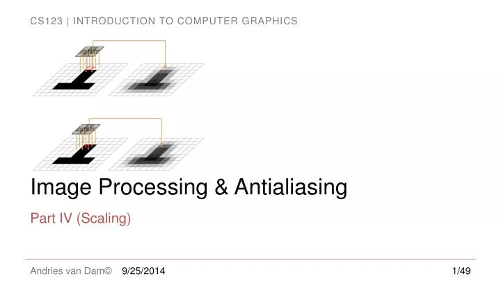
Image Processing & Antialiasing. Part IV (Scaling). Outline. Images & Hardware Example Applications Jaggies & Aliasing Sampling & Duals Convolution Filtering Scaling Reconstruction Scaling, continued Implementation. Review. Theory tells us:

E N D
Image Processing & Antialiasing Part IV (Scaling) 9/25/2014
Outline • Images & Hardware • Example Applications • Jaggies & Aliasing • Sampling & Duals • Convolution • Filtering • Scaling • Reconstruction • Scaling, continued • Implementation 9/25/2014
Review • Theory tells us: • Convolving with sinc in the spatial domain is the optimal filtering • Sampling with a unit comb doesn’t work – need to sample with Dirac delta comb • But sampling with Dirac comb produces infinitely repeating spectra • And they will overlap and cause even more corruption if sampling at or below Nyquist limit • Assuming we use an adequate sampling rate and pre-filter the unrepresentable frequencies, we can use a reconstruction filter to give us a good approximation to the original signal, which we can then scale or otherwise transform, and then re-sample computationally • Actual sampling with a CCD array compounds problems in that it is unweightedarea sampling (box filtering), which produces a corrupted spectrum which is replicated • Solution is filtering to deal as well as possible with all these problems – filters can be combined, as we’ll see 9/25/2014
1D Image Filtering/Scaling Up Again • Once again, consider the following scan-line: • As we saw, if we want to scale up by any rational number a, we must sample every 1/a pixel intervals in the source image • Having shown qualitatively how various filter functions help us resample, let’s get more quantitative: show how one does convolution in practice, using 1D image scaling as driving example 9/25/2014
h ( x ) k x 1 . 5 k ( ) h’ ( k ) h 1 . 5 Resampling for Scaling Up (1/2) • Call continuous reconstructed image intensity function h(x). For triangle filter, it looks as before: • To get intensity of integer pixel k in 1.5X scaled destination image, h’(x), sample reconstructed image h(x) at point • Therefore, intensity function transformed for scaling is: Note: Here we start sampling at the first pixel – slide 21 shows a slightly more accurate algorithm which starts sampling to the left of the first pixel 9/25/2014
Resampling for Scaling Up (2/2) • As before, to build transformed function h’(k), take samples of h(x) at non-integer locations. reconstructed waveform h(x) sample it at 15 real values h(k/1.5) plot it on the integer grid h’(x) 9/25/2014
Resampling for Scaling Up: An Alternate Approach (1/3) • Previous slide shows scaling up by following conceptual process: • reconstruct (by filtering) original continuous intensity function from discrete number of samples • resample reconstructed function at higher sampling rate • stretch our inter-pixel samples back into integer-pixel-spaced range • Alternate conceptualapproach: we can change when we scale and still get same result by first stretching out reconstructed intensity function, then sampling it at integer pixel intervals 9/25/2014
Resampling for Scaling Up : An Alternate Approach (2/3) • This new method performs scaling in second step rather than third: stretches out the reconstructed function rather than the sample locations • reconstruct original continuous intensity function from discrete number of samples • scale up reconstructed function by desired scale factor • sample reconstructed function at integer pixel locations 9/25/2014
Resampling for Scaling Up : An Alternate Approach (3/3) • Alternate conceptual approach (compare to slide 6); practically, we’ll do both steps at the same time anyhow reconstructed waveform h(x) scaled up reconstructed waveform h(x/1.5) plot it on the integer grid h’(x) 9/25/2014
Scaling Down (1/6) Why scaling down is more complex than scaling up • Try same approach as scaling up • reconstruct original continuous intensity function from discrete number of samples, e.g., 15 samples in source (different case from that of 10 samples of source we just used) • scale down reconstructed function by desired scale factor, e.g., 3 • sample reconstructed function (now 3 times narrower), e.g. 5 samples for this case, at integer pixel locations • Unexpected and unwanted side effect: by compressing waveform into 1/3 its original interval, spatial frequencies tripled, which extends (somewhat) band-limited spectrum by factor of 3 in frequency domain. Can’t display these higher frequencies without aliasing! • Back to low pass filtering again. Multiply by box in frequency domain to limit to original frequency band, e.g., when scaling down by 3, low-pass filter to limit frequency band to 1/3 its new width 9/25/2014
Scaling Down (2/6) A sine in the spatial domain… is a spike in the frequency domain Signal compression in the spatial domain… equals frequency expansion in the frequency domain (approx.) box in the frequency domain cuts out high frequencies • Simple sine wave example • First we start with sine wave: • 1/3 Compression of sine wave and expansion of frequency band: • Get rid of new high frequencies (only one here) with low-pass box filter in frequency domain • Only low frequencies will remain 9/25/2014
d) Low-pass filtered, reconstructed, scaled-down signal before re-sampling Scaling Down (3/6) • Same problem for a complex signal (shown in frequency domain) • a) – c) upscaling, d) – e) downscaling • If we shrink the signal in the spatial domain, there is more activity in a smaller space, which increases the spatial frequencies, thus widening the frequency domain representation a) Low-pass filtered, reconstructed , scaled-up signal before re-sampling c) Low pass filtered again, band-limited reconstructed signal e) Scaled-down signal convolved with comb – replicas overlap badlyand low-pass filtering will have bad aliases b) Resampled filtered signal – convolution of spectrum with impulse comb produces replicas 9/25/2014
Scaling Down (4/6) • Revised (conceptual) pipeline for scaling down image: • reconstruction filter: low-pass filter to reconstruct continuous intensity function from old scanned (box-filtered and sampled) image, also gets rid of replicated spectra due to sampling (convolution of spectrum w/ a delta comb) • scale down reconstructed function • scale-down filter: low-pass filter to get rid of newly introduced high frequencies due to scaling down (but it can’t really deal with corruption due to overlapped replications if higher frequencies are too high for Nyquist criterion due to inadequate sampling rate ) • sample scaled reconstructed function at pixel intervals • Now we’re filtering explicitly twice (after scanner implicitly box filtered) • first to reconstruct signal (filter g1) • then to low-pass filter high frequencies in scaled-down version (filter g2) 9/25/2014
Scaling Down (5/6) • In actual implementation, we can combine reconstruction and frequency band-limiting into one filtering step. Why? • Associativity of convolution: • Convolve our reconstruction and low-pass filters together into one combined filter! • Result is simple: convolution of two sinc functions is just the larger sinc function. In our case, approximate larger sinc with larger triangle, and convolve only once with it. • Theoretical optimalsupport for scaling up is 2, but for down-scaling by a is 2/a, i.e., >2 • Why does support >2 for down-scaling make sense from an information preserving PoV? 9/25/2014
Scaling Down (6/6) Why does complex-sounding convolution of two differently-scaled sinc filters have such simple solution? • Convolution of two sinc filters in spatial domain sounds complicated, but remember that convolution in the spatial domain means multiplication in the frequency domain! • A sinc in the spatial domain is a box in the frequency domain. Multiplication of two boxes is easy— product is narrower of two pulses: • Narrower pulse in frequency domain is wider sinc in spatial domain (lower frequencies) • Thus, instead of filtering twice (once for reconstruction, once for low-pass), just filter once with wider of two filters to do the same thing • True for sinc or triangle approximation—it is the width of the support that matters 9/25/2014
Outline • Images & Hardware • Example Applications • Jaggies & Aliasing • Sampling & Duals • Convolution • Filtering • Scaling • Reconstruction • Scaling, continued • Implementation 9/25/2014
Algebraic Reconstruction (1/2) • So far textual explanations; let’s get algebraic! • Let f’(x) be the theoretical, continuous, box-filtered (thus corrupted) version of original continuous image function f(x) • produced by scanner just prior to sampling • Reconstructed, doubly-filtered image intensity function h(x) returns image intensity at sample location x, where x is real (and determined by backmapping using the scaling ratio); it is convolution of f’(x) with filter g(x) that is the wider of the reconstruction and scaling filters, centered at x : • But we want to do the discrete convolution, and regardless of where the back-mapped x is, only look at nearby integer locations where we have actual pixel values 9/25/2014
Algebraic Reconstruction (2/2) • Only need to evaluate the discrete convolution at pixel locations since that's where the function’s value will be displayed • Replace integral with finite sum over pixel locations covered by filter g(x) centered at x. • Thus convolution reduces to: • Note: sign of argument of g does not matter since our filters are symmetric, e.g., triangle • e.g., if x = 13.7, and a triangle filter has optimal scale-up supportof 2, evaluate g(13 -13.7) = 0.3 and g(14 – 13.7) = 0.7and multiply those weights by the values of pixels 13 and 14respectively For all pixels i falling under filter support centered at x Filter value at pixel location i Pixel value at i 9/25/2014
Unified Approach to Scaling Up and Down • Scaling up has constant reconstruction filter, support = 2 • Scaling down has support 2/a where a is the scale factor • Can parameterize image functions with scale: write a generalized formula for scaling up and down • g(x, a) is parameterized filter function; • The filter function now depends on the scale factor, a, because the support width and filter weights change when downscaling by different amounts. (g does not depend on a when up-scaling.) • h(x, a) is reconstructed, filtered intensity function (either ideal continuous, or discrete approximation) • h’(k, a) is scaled version of h(x, a) dealing with image scaling, sampled at pixel values of x = k 9/25/2014
Image intervals • In order to handle edge cases gracefully, we need to have a bit of insight about images, specifically the interval around them. • Suppose we sample at each integer mark on the function below. • Consider the interval around each sample point. i.e. the interval for which the sample represents the original function. What should it be? • Each sample’s interval must have width one • Notice that this interval extends past the lower and upper indices (0 and 4) • For a function with pixel values P0, P1,…,P4, , the domain is not [0, 4], but [-0.5, 4.5]. • Intuition: Each pixel “owns” a unit interval around it. Pixel P1, owns [0.5, 1.5] -.5 .5 1.5 2.5 3.5 4.5 0 1 2 3 4 9/25/2014
Correct back-mapping (1/2) • When we back-map we want: • start of the destination interval start of source interval • end of destination interval end of the source interval. • The question then is, where do we back-map points within the destination image? • we want there to be a linear relationship in our back-map () • This results in the system of linear equations: Source P1 P2 Destination q2 q1 k-1+.5 -.5 … Pk-1 P0 -.5 … qm-1 q0 k = size of source image m = size of destination image m-1+.5 9/25/2014
k = size of source image m = size of destination image Correct back-mapping (2/2) • Solving the system of equations give us… This equation tells us where to center the filter when scaling an image. Does not solve the problem of having to renormalize the weights when filter goes off the edge. 9/25/2014
Reconstruction for Scaling • Just as filter is a continuous function of x and a (scale factor), so too is the filtered image function h(x, a) • Back-map destination pixel at k to (non-integer) source location • Can almost write this sum out as code but still need to figure out summation limits and filter function Filter g, centered at sample point x, evaluated at i For all pixels i where i is in support of g Pixel at integer i 9/25/2014
Nomenclature Summary • Nomenclature summary: • f’(x) is original, mostly band-limited, continuous intensity function – never produced in practice! • Piis sampled (box-filtered, comb multiplied) f’(x) stored as pixel values • g(x, a)is parameterized filter function, wider of the reconstruction and scaling filters, removing both replicas due to sampling and higher frequencies due to frequency multiplication if downscaling • h(x, a)is reconstructed, filtered intensity function (either ideal continuous or discrete approximate) • h’(k, a)is scaled version of h(x, a)dealing with image scaling • a is scale factor • k is index of a pixel in the destination image • In code, you will be starting with Pi(input image) and doing the filtering and mapping in one step to get h’(x, a), the output image 9/25/2014
Two for the Price of One (1/2) Min(a,1) Max(1/a,1) -Max(1/a,1) • Triangle filter, modified to be reconstruction for scaling by factor of a: • for a> 1, looks just like the old triangle function. Support is 2 and the area is 1 • For a < 1, it’s vertically squashed and horizontally stretched. Support is 2/a and the area again is 1. • Careful… • this function will be called a lot. Can you optimize it? • remember: fabs() is just floating point version of abs() 9/25/2014
Scale up left = ceil( c–1) Scale down right = floor( c+ 1) c- 1/a c c+1/a _ 1 left = ceil( c –) a c- 1 c+ 1 1 _ right = floor(c+ ) a Two for the Price of One (2/2) • The pseudocode tells us support of g • a < 1: (-1/a) ≤ x ≤ (1/a) • a ≥ 1: -1 ≤ x ≤ 1 • Can describe leftmost and rightmost pixels that need to be examined for pixel k in destination image as delimiting a window around the center, . Window is size 2 for scaling up and 2/a for scaling down. • Note is not, in general, an integer. Yet we want to use integer index for the pixel array. Use floor() and ceil(). • If a > 1 (scale up) • If a < 1 (scale down) 9/25/2014
Triangle Filter Pseudocode double h-prime(intk, double a) { double sum = 0, weights_sum = 0; int left, right; float support; float center= k/a + (1-a)/2; support = (a > 1) ? 1 : 1/a; left = ceil(center – support); right = floor(center + support); for (int i = left; i <= right, i++) { sum += g(i – center, a) * orig_image.Pi; weights_sum += g(i – center, a); } result = sum/weights_sum; } To ponder: When don’t you need to normalize sum? Why? How can you optimize this code? Remember to bound check! 9/25/2014
The Big Picture, Algorithmically Speaking • For each pixel in destination image: • determine which pixels in source image are relevant • by applying techniques described above, use values of source image pixels to generate value of current pixel in destination image 9/25/2014
Normalizing Sum of Filter Weights (1/5) • Notice in pseudocode that we sum filter weights, then normalize sum of weighted pixel contributions by dividing by filter weight sum. Why? • Because non-integer width filters produce sums of weights which vary as a function of sampling position. Why is this a problem? • “Venetian blinds” – sums of weights increase and decrease away from 1.0 regularly across image. • These “bands” scale image with regularly spaced lighter and darker regions. • First we will show example of why filters with integer radii do sum to 1 and then why filters with real radii may not 9/25/2014
Normalizing Sum of Filter Weights (2/5) • Verify that integer-width filters have weights that always sum to one: notice that as filter shifts, one weight may be lowered, but it has a corresponding weight on opposite side of filter, a radius apart, that increases by same amount If we slide the filter 0.25 units to the right, we have effectively slid the two pixels under it by 0.25 units to the left relative to it. Since the pixels move by the same amount, an increase on one side of the filter will be perfectly compensated for by a decrease on the other. Our weights again sum to 1.0. When we place the filter halfway between two pixels, we get two weights, each 0.5. The symmetry of pixel placement ensures that we will get identical values on each side of the filter. The two weights again sum to 1.0 When we place it directly over a pixel, we have one weight, and it is exactly 1.0. Therefore, the sum of weights (by definition) is 1.0 Consider our familiar triangle filter 9/25/2014
Normalizing Sum of Filter Weights (3/5) But when filter radius is non-integer, sum of weights changes for different filter positions In this example, first position filter (radius 2.5) at location A. Intersection of dotted line at pixel location with filter determines weight at that location. Now consider filter placed slightly right of A, at B. Differences in new/old pixel weights shown as additions or subtractions. Because filter slopes are parallel, these differences are all same size. But there are 3 negative differences and 2 positive, hence two sums will differ 9/25/2014
Normalizing Sum of Filter Weights (4/5) • When radius is an integer, contributing pixels can be paired and contribution from each pair is equal. The two pixels of a pair are at a radius distance from each other • Proof: see equation for value of filter with radius r centered at non-integer location d: • Suppose pair is (b, c) as in figure to right. Contribution sum becomes: • (Note |d – c| = x and |d – b| = r – x) r=2 b d c 9/25/2014
Normalizing Sum of Filter Weights (5/5) • Sum of contributions from two pixels in a pair does not depend on d (location of filter center) • Sum of contributions from all pixels under filter will not vary, no matter where we’re reconstructing • For integer width filters, we do not need to normalize • When scaling up, we always have integer-width filter, so we don’t need to normalize! • When scaling down, our filter width is generally non-integer, and we do need to normalize. • Can you rewrite the pseudocode to take advantage of this knowledge? 9/25/2014
Scaling in 2D – Two Methods • We know how to do 1D scaling, but how do we generalize to 2D? • Do it in 2D “all at once” with one generalized filter • Harder to implement • More general • Generally more “correct” – deals with high frequency “diagonal” information • Do it in 1D twice – once to rows, once to columns • Easy to implement • For certain filters, works pretty decently • Requires intermediate storage • What’s the difference? 1D is easier, but is it a legitimate solution? 9/25/2014
Digression on Separable Kernels (1/2) • The 1D two-pass method and the 2D method will give the same result if and only ifthe filter kernel (pixel mask) is separable • A separable kernel is one that can be represented as a product of two vectors. Those vectors would be your 1D kernels. • Mathematically, a matrix is separable if its rank (number of linearly independent rows/columns) is 1 • Examples: box, Gaussian, Sobel (edge detection), but not cone and pyramid • Otherwise, there is no way to split a 2D filter into 2 1D filters that will give the same result 9/25/2014
Digression on Separable Kernels (2/2) • For your assignment, the 1D two-pass approach suffices and is easier to implement. It does not matter whether you apply the filter in the x or y direction first. • Recall that ideally we use a sinc for the low pass filter, but can’t in practice, so use, say, pyramid or Gaussian. • Pyramid is not separable, but Gaussian is • Two 1D triangle kernels will not make a square 2D pyramid, but it will be close • If you multiply [0.25, 0.5, 0.25]T * [0.25, 0.5, 0.25], you get the kernel on slide 40, which is not a pyramid – the pyramid would have identical weights around the border! See also next slide… • Feel free to use 1D triangles as an approximation to an approximation in your project 9/25/2014
Pyramid vs. Triangles • Not the same, but close enough for a reasonable approximation 2D Pyramid kernel 2D kernel from two 1D triangles 9/25/2014
Examples of Separable Kernels Gaussian Box PSF is the Point Spread Response, same as your filter kernel http://www.dspguide.com/ch24/3.htm 9/25/2014
Why is Separable Faster? • Why is filtering twice with 1D filters faster than once with 2D? • Consider your image with size W x Hand a 1D filter kernel of width F • Your equivalent 2D filter with have a size F2 • With your 1D filter, you will need to do F multiplications and adds per pixel and run through the image twice (e.g., first horizontally (saved in a temp) and then vertically) • Roughly 2FWH calculations • With your 2D filter, you need to do F2 multiplications and adds per pixel and go through the image once • Roughly F2WH calculations • Using a 1d filter, the difference is about 2/F times the computation time • As your filter kernel size gets larger, the gains from a separable kernel become more significant! (at the cost of the temp, but that’s not an issue for most systems these days…) 9/25/2014
Digression on Precomputed Kernels • Certain mapping operations (such as image blurring, sharpening, edge detection, etc.) change values of destination pixels, but don’t remap pixel locations, i.e., don’t sample between pixel locations. Their filters can be precomputed as a “kernel” (or “pixel mask”) • Other mappings, such as image scaling, require sampling between pixel locations and therefore calculating actual filter values at those arbitrary non-integer locations. For these operations, often easier to approximate pyramid filter by applying triangle filters twice, once along x-axis of source, once along y-axis 9/25/2014
Precomputed Filter Kernels (1/3) • Filter kernel is an array of filter values precomputed at predefined sample points • Kernels are usually square, odd number by odd number size grids (center of kernel can be at pixel that you are working with [e.g. 3x3 kernel shown here]): • Why does precomputation only work for mappings which sample only at integer pixel intervals in original image? • If filter location is moved by fraction of a pixel in source image, pixels fall under different locations within filter, correspond to different filter values. • Can’t precompute for this since infinitely many non-integer values • Since scaling will almost always require non-integer pixel sampling, you cannot use precomputed kernels. However, they will be useful for image processing algorithms such as edge detection. 9/25/2014
Precomputed Filter Kernels (2/3) Evaluating the kernel • To evaluate, place kernel’s center over integer pixel location to be sampled. Each pixel covered by kernel is multiplied by corresponding kernel value; results are summed • Note: have not dealt with boundary conditions. One common tactic is to act as if there is a buffer zone where the edge values are repeated 9/25/2014
Precomputed Filter Kernels (3/3) Filter kernel in operation • Pixel in destination image is weighted sum of multiple pixels in source image 9/25/2014
Pixel at row/column intersection Supersampling for Image Synthesis (1/2) • Anti-aliasing of primitives in practice • Bad Old Days: Generate low-res image and post-filter the whole image, e.g. with pyramid – blurs image (with its aliases – bad crawlies) • Alternative: super-sample and post-filter, to approximate pre-filtering before sampling • Pixel’s value computed by taking weighted average of several point samples around pixel’s center. Again, approximating (convolution) integral with weighted sum • Stochastic (random) point sampling as an approximation converges faster and is more correct than equally spaced grid sampling Center of current pixel samples can be taken in grid around pixel center… or they can be taken at random locations 9/25/2014
Supersampling for Image Synthesis (2/2) • Why does supersampling work? • Sampling a higher frequency pushes the replicas apart, and since spectra fall off at approximately 1/f pfor (1 < p < 2) (i.e. somewhere between linearly and quadratically), the tails overlap much less, causing much less corruption before the low-pass filtering • With fewer than 128 distinguishable levels of intensity, being off by one step is hardly noticeable • Stochastic sampling may introduce some random noise, but if you make multiple passes it will eventually converge on the correct answer • Since you need to take multiple samples and filter them, this process is computationally expensive 9/25/2014
Modern Anti-Aliasing Techniques – Postprocessing • Ironically, current trends in graphics are moving back toward anti-aliasing as a post processing step • AMD’s MLAA (Morphological Anti-Aliasing) and nVidia’s FXAA (Fast Approximate Anti-Aliasing) plus many more • General idea: find edges/silhouettes in the image, slightly blur those areas • Faster and lower memory requirements compared to supersampling • Scales better with larger resolutions • Compared to just plain blur filtering, looks better due to intelligently filtering along contours in the image. There is more filtering in areas of bad aliasing while still preserving crispness. 9/25/2014
MLAA Example 9/25/2014
FXAA Example 9/25/2014
MLAA vs. Blur Filter 9/25/2014