Download
1 / 42
420 likes | 435 Views
CS380: Computer Graphics Screen Space & World Space. Sung-Eui Yoon ( 윤성의 ). Course URL: http://sglab.kaist.ac.kr/~sungeui/CG. Class Objectives. Understand different spaces and basic OpenGL commands Understand a continuous world, Julia sets. Your New World.

E N D
CS380: Computer Graphics Screen Space & World Space Sung-Eui Yoon (윤성의) Course URL: http://sglab.kaist.ac.kr/~sungeui/CG
Class Objectives • Understand different spaces and basic OpenGL commands • Understand a continuous world, Julia sets
Your New World • A 2D square ranging from (-1, -1) to (1, 1) • You can draw in the box with just a few lines of code
Code Example (Immediate Mode) Legacy OpenGL code: glColor3d(0.0, 0.8, 1.0); glBegin(GL_POLYGON); glVertex2d(-0.5, -0.5); glVertex2d( 0.5, -0.5); glVertex2d( 0.5, 0.5); glVertex2d(-0.5, 0.5); glEnd();
OpenGL Command Syntax • glColor3d(0.0, 0.8, 1.0);
OpenGL Command Syntax • You can use pointers or buffers • Using buffers for drawing is much more efficient glColor3f(0.0, 0.8, 1.0); GLfloat color_array [] = {0.0, 0.8, 1.0}; glColor3fv (color_array);
Another Code Example OpenGL Code: glColor3d(0.0, 0.8, 1.0); glBegin(GL_POLYGON); glVertex2d(-0.5, -0.5); glVertex2d( 0.5, -0.5); glVertex2d( 0.5, 0.5); glEnd()
Drawing Primitives in OpenGL The red book
Yet Another Code Example OpenGL Code:glColor3d(0.8, 0.6, 0.8); glBegin(GL_LINE_LOOP); for (i = 0; i < 360;i = i + 2) { x = cos(i*pi/180); y = sin(i*pi/180); glVertex2d(x, y); } glEnd();
OpenGL as a State Machine • OpenGL maintains various states until you change them // set the current color state glColor3d(0.0, 0.8, 1.0); glBegin(GL_POLYGON); glVertex2d(-0.5, -0.5); glVertex2d( 0.5, -0.5); glVertex2d( 0.5, 0.5); glEnd()
OpenGL as a State Machine • OpenGL maintains various states until you change them • Many state variables refer to modes (e.g., lighting mode) • You can enable, glEnable (), or disable, glDisable () • You can query state variables • glGetFloatv (), glIsEnabled (), etc. • glGetError (): very useful for debugging
Debugging Tip #define CheckError(s) \ { \ GLenum error = glGetError(); \ if (error) \ printf("%s in %s\n",gluErrorString(error),s); \ } glTexCoordPointer (2, x, sizeof(y), (GLvoid *) TexDelta); CheckError ("Tex Bind"); glDrawElements(GL_TRIANGLES, x, GL_UNSIGNED_SHORT, 0); CheckError ("Tex Draw");
OpenGL Ver. 4.3 (Using Retained Mode) ShaderInfo shaders[] = { { GL_VERTEX_SHADER, "triangles.vert" }, { GL_FRAGMENT_SHADER, "triangles.frag" }, { GL_NONE, NULL } }; GLuint program = LoadShaders(shaders); glUseProgram(program); glVertexAttribPointer(vPosition, 2, GL_FLOAT, GL_FALSE, 0, BUFFER_OFFSET(0)); glEnableVertexAttribArray(vPosition); } Void display(void) { glClear(GL_COLOR_BUFFER_BIT); glBindVertexArray(VAOs[Triangles]); glDrawArrays(GL_TRIANGLES, 0, NumVertices); glFlush(); } Int main(int argc, char** argv) { glutInit(&argc, argv); glutInitDisplayMode(GLUT_RGBA); glutInitWindowSize(512, 512); glutInitContextVersion(4, 3); glutInitContextProfile(GLUT_CORE_PROFILE); glutCreateWindow(argv[0]); if (glewInit()) { exit(EXIT_FAILURE); } init();glutDisplayFunc(display); glutMainLoop(); } #include <iostream> using namespace std; #include "vgl.h" #include "LoadShaders.h" enum VAO_IDs { Triangles, NumVAOs }; enum Buffer_IDs { ArrayBuffer, NumBuffers }; enum Attrib_IDs { vPosition = 0 }; GLuint VAOs[NumVAOs]; GLuint Buffers[NumBuffers]; const GLuint NumVertices = 6; Void init(void) { glGenVertexArrays(NumVAOs, VAOs); glBindVertexArray(VAOs[Triangles]); GLfloat vertices[NumVertices][2] = { { -0.90, -0.90 }, // Triangle 1 { 0.85, -0.90 }, { -0.90, 0.85 }, { 0.90, -0.85 }, // Triangle 2 { 0.90, 0.90 }, { -0.85, 0.90 } }; glGenBuffers(NumBuffers, Buffers); glBindBuffer(GL_ARRAY_BUFFER, Buffers[ArrayBuffer]); glBufferData(GL_ARRAY_BUFFER, sizeof(vertices), vertices, GL_STATIC_DRAW);
Classic Rendering Pipeline Transformation: Vertex processing Rasterization: Pixel processing CPU GPU
Prepare vertex array data Program on vertex: Model, View, Projection transforms Vertex processing Subdivide (optional) Catmull-Clark subdivision Ack. OpenGL and wiki
Prepare vertex array data Program on vertex: Model, View, Projection transforms Vertex processing Subdivide (optional) Primitive clipping, perspective divide, viewport transform Face culling Depth test Fragment processing Ack. OpenGL and wiki
Study a visualization of a simple iterative function defined over the imaginary plane It has chaotic behavior Small changes have dramatic effects Julia Sets (Fractal) Demo
Julia Set - Definition • The Julia set Jc for a number c in the complex plane P is given by: Jc = { p | pP and pi+1 = p2i + c converges to a fixed limit }
Complex Numbers • Consists of 2 tuples (Real, Imaginary) • E.g., c = a + bi • Various operations • c1 + c2 = (a1 + a2) + (b1 + b2)i • c1 c2 = (a1a2 - b1b2) + (a1b2 + a2b1)i • (c1)2 = ((a1)2 – (b1)2) + (2 a1b1)i • |c| = sqrt(a2 + b2)
Convergence Example • Real numbers are a subset of complex numbers: • Consider c = [0, 0], and p = [x, 0] • For what values of x is xi+1 = xi2 convergent? How about x0 = 0.5? x0-4 = 0.5, 0.25, 0.0625, 0.0039
Convergence Example • Real numbers are a subset of complex numbers: • consider c = [0, 0], and p = [x, 0] • for what values of x is xi+1 = xi2 convergent? How about x0 = 1.1? x0-4 = 1.1, 1.21, 1.4641, 2.14358 0 1
Convergence Properties • Suppose c = [0,0], for what complex values of p does the series converge? • For real numbers: • If |xi| > 1, then the series diverges • For complex numbers • If |pi| > 2, then the series diverges • Loose bound Imaginary part Real part The black points are the ones in Julia set
A Peek at the Fractal Code class Complex { float re, im; }; viod Julia (Complex p, Complex c, int & i, float & r) { int maxIterations = 256; for (i = 0; i < maxIterations;i++) { p = p*p + c; rSqr = p.re*p.re + p.im*p.im; if( rSqr > 4 ) break; } r = sqrt(rSqr); } i & r are used to assign a color
How can we see more? • Our world view allows us to see so much • What if we want to zoom in? • We need to define a mapping from our desired world view to our screen
Mapping from World to Screen Camera Window World Monitor Screen
Screen Space • Graphical image is presented by setting colors for a set of discrete samples called “pixels” • Pixels displayed on screen in windows • Pixels are addressed as 2D arrays • Indices are “screen-space” coordinates (width-1,0) (0,0) (0,height-1) (width-1, height-1)
OpenGL Coordinate System (0,0) (width-1,0) (0, height-1) (width-1, height-1) (0,0) Windows Screen Coordinates OpenGL Screen Coordinates
Pixel Independence • Often easier to structure graphical objects independent of screen or window sizes • Define graphical objects in “world-space” 1.25 meters 500 cubits 2 meters 800 cubits
1 -1 1 -1 Normalized Device Coordinates • Intermediate “rendering-space” • Compose world and screen space • Sometimes called “canonical screen space”
Why Introduce NDC? • Simplifies many rendering operations • Clipping, computing coefficients for interpolation • Separates the bulk of geometric processing from the specifics of rasterization (sampling) • Will be discussed later
Mapping from World to Screen NDC Window World Screen xs xw xn
xn? xw World Space to NDC 1 w.t -1 w.b -1 w.l 1 w.r
NDC to Screen Space xs xn • Same approach • Solve for xs origin.y1 height -1 width origin.x -1 1
Class Objectives were: • Understand different spaces and basic OpenGL commands • Understand a continuous world, Julia sets
Any Questions? • Come up with one question on what we have discussed in the class and submit at the end of the class • 1 for already answered questions • 2 for typical questions • 3 for questions with thoughts or that surprised me • Submit at least four times during the whole semester • Multiple questions in one time are counted as once
Homework • Go over the next lecture slides before the class • Watch 2 SIGGRAPH videos and submit your summaries before every Tue. class • Send an email to cs380ta@gmail.com • Just one paragraph for each summary Example: Title: XXX XXXX XXXX Abstract: this video is about accelerating the performance of ray tracing. To achieve its goal, they design a new technique for reordering rays, since by doing so, they can improve the ray coherence and thus improve the overall performance.
Homework for Next Class • Read Chapter 1, Introduction • Read “Numerical issues” carefully
Next Time • Basic OpenGL program structure and how OpenGL supports different spaces
Mapping from World to Screen in OpenGL NDC Window Camera Viewport World Screen xs xw xn
Screen Cooridnates NDC Window World Screen xs xw xn
(0,0) (width-1,0) (0, height-1) (width-1, height-1) (0,0) Windows Screen Coordinates OpenGL Screen Coordinates