Ocean circulation estimations using GOCE gravity field models

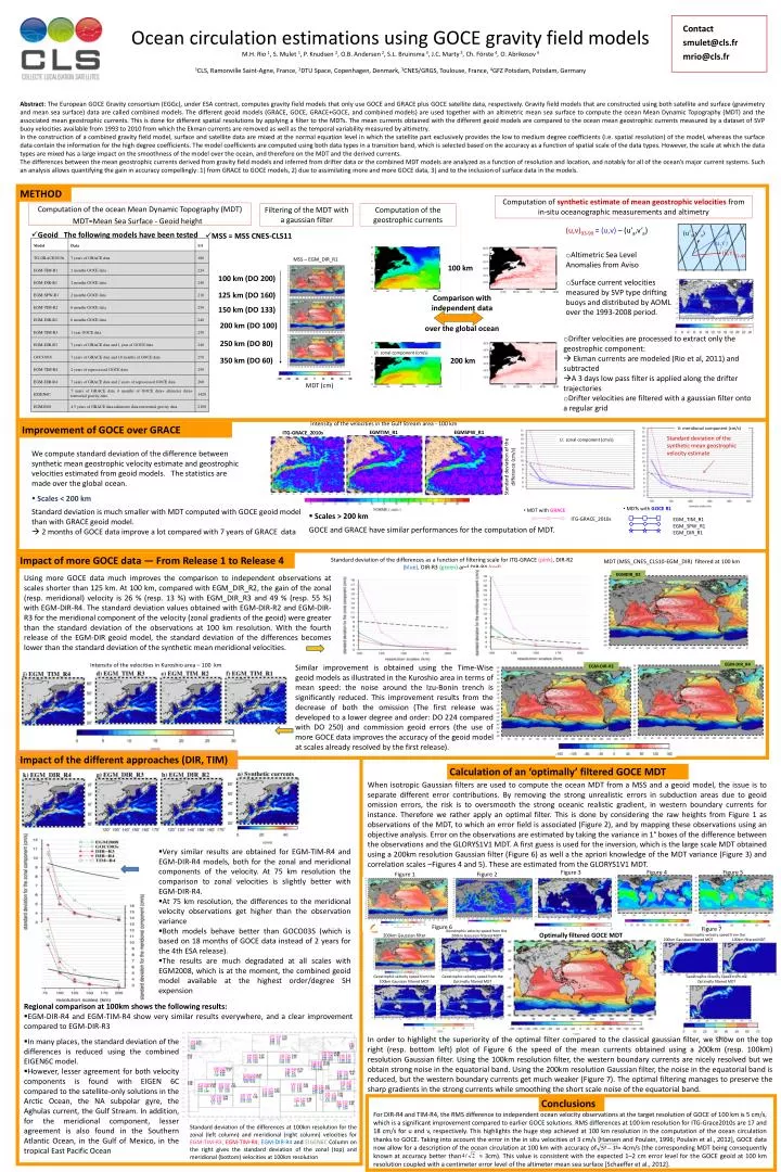
1. (u’a,v’a) (u,v) Contact smulet@cls.fr mrio@cls.fr Ocean circulation estimations using GOCE gravity field models • M.H. Rio 1, S. Mulet 1, P. Knudsen 2, O.B. Andersen 2, S.L. Bruinsma 3, J.C. Marty 3, Ch. Förste 4, O. Abrikosov 4 • 1CLS, Ramonville Saint-Agne, France, 2DTU Space, Copenhagen, Denmark, 3CNES/GRGS, Toulouse, France, 4GFZ Potsdam, Potsdam, Germany Abstract: The European GOCE Gravity consortium (EGGc), under ESA contract, computes gravity field models that only use GOCE and GRACE plus GOCE satellite data, respectively. Gravity field models that are constructed using both satellite and surface (gravimetry and mean sea surface) data are called combined models. The different geoid models (GRACE, GOCE, GRACE+GOCE, and combined models) are used together with an altimetric mean sea surface to compute the ocean Mean Dynamic Topography (MDT) and the associated mean geostrophic currents. This is done for different spatial resolutions by applying a filter to the MDTs. The mean currents obtained with the different geoid models are compared to the ocean mean geostrophic currents measured by a dataset of SVP buoy velocities available from 1993 to 2010 from which the Ekman currents are removed as well as the temporal variability measured by altimetry. In the construction of a combined gravity field model, surface and satellite data are mixed at the normal equation level in which the satellite part exclusively provides the low to medium degree coefficients (i.e. spatial resolution) of the model, whereas the surface data contain the information for the high degree coefficients. The model coefficients are computed using both data types in a transition band, which is selected based on the accuracy as a function of spatial scale of the data types. However, the scale at which the data types are mixed has a large impact on the smoothness of the model over the ocean, and therefore on the MDT and the derived currents. The differences between the mean geostrophic currents derived from gravity field models and inferred from drifter data or the combined MDT models are analyzed as a function of resolution and location, and notably for all of the ocean’s major current systems. Such an analysis allows quantifying the gain in accuracy compellingly: 1) from GRACE to GOCE models, 2) due to assimilating more and more GOCE data, 3) and to the inclusion of surface data in the models. METHOD Computation of synthetic estimate of mean geostrophic velocities from in-situ oceanographic measurements and altimetry Computation of the oceanMeanDynamicTopography (MDT) Filtering of the MDT with a gaussian filter Computation of the geostrophic currents 100 km MDT=MeanSeaSurface - Geoidheight • Geoid The followingmodels have been tested (u,v)93-99 =(u,v) – (u’a,v’a) • MSS = MSS CNES-CLS11 Comparison withindependent data over the global ocean • Altimetric Sea Level Anomalies from Aviso MSS – EGM_DIR_R1 100 km (DO 200) • Surface current velocities measured by SVP type drifting buoys and distributed by AOML over the 1993-2008 period. 125 km (DO 160) 150 km (DO 133) 200 km 200 km (DO 100) • Drifter velocities are processed to extractonly the geostrophic component: •  Ekmancurrents are modeled (Rio et al, 2011) and subtracted • A 3 dayslowpassfilterisappliedalong the drifter trajectories • Drifter velocities are filteredwith a gaussianfilter onto a regulargrid 250 km (DO 80) 350 km (DO 60) MDT (cm) • MDTswithGOCER1 EGM_TIM_R1 EGM_SPW_R1 EGM_DIR_R1 Intensity of the velocities in the Gulf Stream area - 100 km Improvement of GOCE over GRACE V: meridional component (cm/s) EGMTIM_R1 EGMSPW_R1 ITG-GRACE_2010s Standard deviation of the synthetic mean geostrophic velocity estimate U: zonal component (cm/s) • MDT withGRACE ITG-GRACE_2010s Wecompute standard deviation of the differencebetweensyntheticmeangeostrophicvelocityestimate and geostrophicvelocitiesestimatedfromgeoidmodels. The statistics are made over the global ocean. U: zonal component (cm/s) • Scales < 200 km • Standard deviationismuchsmallerwith MDT computedwith GOCE geoid model thanwith GRACE geoid model. •  2 months of GOCE data improve a lot comparedwith 7 years of GRACE data • Scales > 200 km • GOCE and GRACE have similar performances for the computation of MDT. Impact of more GOCE data ― FromRelease 1 to Release 4 Standard deviation of the differences as a function of filteringscale for ITG-GRACE (pink), DIR-R2 (blue), DIR-R3 (green) and DIR-R4 (red) MDT (MSS_CNES_CLS10-EGM_DIR) filteredat 100 km EGMDIR_R2 Using more GOCE data much improves the comparison to independent observations at scales shorter than 125 km. At 100 km, compared with EGM_DIR_R2, the gain of the zonal (resp. meridional) velocity is 26 % (resp. 13 %) with EGM_DIR_R3 and 49 % (resp. 55 %) with EGM-DIR-R4. The standard deviation values obtained with EGM-DIR-R2 and EGM-DIR-R3 for the meridional component of the velocity (zonal gradients of the geoid) were greater than the standard deviation of the observations at 100 km resolution. With the fourth release of the EGM-DIR geoid model, the standard deviation of the differences becomes lower than the standard deviation of the synthetic mean meridional velocities. EGMDIR_R2 Standard deviation of the difference (cm/s) Intensity of the velocities in Kuroshio area – 100 km EGM-DIR_R4 Similar improvement is obtained using the Time-Wise geoid models as illustrated in the Kuroshio area in terms of mean speed: the noise around the Izu-Bonin trench is significantly reduced. This improvement results from the decrease of both the omission (The first release was developed to a lower degree and order: DO 224 compared with DO 250) and commission geoid errors (the use of more GOCE data improves the accuracy of the geoid model at scales already resolved by the first release). EGM-DIR-R3 Impact of the differentapproaches (DIR, TIM) Calculation of an ‘optimally’ filtered GOCE MDT When isotropic Gaussian filters are used to compute the ocean MDT from a MSS and a geoid model, the issue is to separate different error contributions. By removing the strong unrealistic errors in subduction areas due to geoid omission errors, the risk is to oversmooth the strong oceanic realistic gradient, in western boundary currents for instance. Therefore we rather apply an optimal filter. This is done by considering the raw heights from Figure 1 as observations of the MDT, to which an error field is associated (Figure 2), and by mapping these observations using an objective analysis. Error on the observations are estimated by taking the variance in 1° boxes of the difference between the observations and the GLORYS1V1 MDT. A first guess is used for the inversion, which is the large scale MDT obtained using a 200km resolution Gaussian filter (Figure 6) as well a the apriori knowledge of the MDT variance (Figure 3) and correlation scales –Figures 4 and 5). These are estimated from the GLORYS1V1 MDT. • Verysimilarresults are obtained for EGM-TIM-R4 and EGM-DIR-R4 models, both for the zonal and meridional components of the velocity. At 75 km resolution the comparison to zonal velocitiesisslightlybetterwith EGM-DIR-R4. • At 75 km resolution, the differences to the meridionalvelocity observations gethigherthan the observation variance • Bothmodelsbehavebetterthan GOCO03S (whichisbased on 18 months of GOCE data instead of 2 years for the 4th ESA release). • The results are muchdegradatedat all scaleswith EGM2008, whichisat the moment, the combinedgeoid model availableat the highestorder/degree SH expension Figure 3 Figure 4 Figure 5 Figure 1 Figure 2 Figure 6 Figure 7 Geostrophicvelocity speed from the 200km Gaussianfiltered MDT Optimallyfiltered GOCE MDT Geostrophicvelocity speed from the 200km Gaussianfiltered MDT 100km filtered MDT 200km Gaussianfilter Geostrophicvelocity speed from the 100km Gaussianfiltered MDT Geostrophicvelocity speed from the Optimallyfiltered MDT Geostrophicvelocity speed from the Optimallyfiltered MDT • Regionalcomparisonat 100km shows the followingresults: • EGM-DIR-R4 and EGM-TIM-R4 show verysimilarresultseverywhere, and a clearimprovementcompared to EGM-DIR-R3 In order to highlight the superiority of the optimal filter compared to the classical gaussian filter, we show on the top right (resp. bottom left) plot of Figure 6 the speed of the mean currents obtained using a 200km (resp. 100km) resolution Gaussian filter. Using the 100km resolution filter, the western boundary currents are nicely resolved but we obtain strong noise in the equatorial band. Using the 200km resolution Gaussian filter, the noise in the equatorial band is reduced, but the western boundary currents get much weaker (Figure 7). The optimal filtering manages to preserve the sharp gradients in the strong currents while smoothing the short scale noise of the equatorial band. • In many places, the standard deviation of the differencesisreducedusing the combined EIGEN6C model. • However, lesser agreement for bothvelocity components isfoundwith EIGEN 6C compared to the satellite-only solutions in the ArcticOcean, the NA subpolargyre, the Aghulascurrent, the Gulf Stream. In addition, for the meridional component, lesser agreement isalsofound in the Southern Atlantic Ocean, in the Gulf of Mexico, in the tropical East Pacific Ocean Conclusions For DIR-R4 and TIM-R4, the RMS difference to independent ocean velocity observations at the target resolution of GOCE of 100 km is 5 cm/s, which is a significant improvement compared to earlier GOCE solutions. RMS differences at 100 km resolution for ITG-Grace2010s are 17 and 18 cm/s for u and v, respectively. This highlights the huge step achieved at 100 km resolution in the computation of the ocean circulation thanks to GOCE. Taking into account the error in the in situ velocities of 3 cm/s [Hansen and Poulain, 1996; Poulain et al., 2012], GOCE data now allow for a description of the ocean circulation at 100 km with accuracy of ≈ 4cm/s (the corresponding MDT being consequently known at accuracy better than ≈ 3cm). This value is consistent with the expected 1–2 cm error level for the GOCE geoid at 100 km resolution coupled with a centimeter error level of the altimeter mean sea surface [Schaeffer et al., 2012]. Standard deviation of the differencesat 100km resolution for the zonal (leftcolumn) and meridional (right column) velocities for EGM-TIM-R3, EGM-TIM-R4, EGM-DIR-R4 and EIGEN6C Column on the right gives the standard deviation of the zonal (top) and meridional (bottom) velocitiesat 100km resolution