Download
1 / 85
850 likes | 1.09k Views
Tuesday – AB. Morning (Part 1) Developing Understanding of the Derivative Upload TI 84 Programs Break Morning (Part 2) Ideas That Can Be Explored Before Working with Formulas Connecting Graphs of f, f’, and f” Connecting Differentiability with Continuity Local Linearity. Lunch

E N D
Tuesday – AB • Morning (Part 1) • Developing Understanding of the Derivative • Upload TI 84 Programs • Break • Morning (Part 2) • Ideas That Can Be Explored Before Working with Formulas • Connecting Graphs of f, f’, and f” • Connecting Differentiability with Continuity • Local Linearity • Lunch • Afternoon (Part 1) • Share an Activity • Calculus Games • Discussion of Homework Problems • Break • Afternoon (Part 2) • Slope Fields • Reasoning with Tabular Data
Tuesday Assignment - AB • Multiple Choice Questions on the 2013 test: 3, 6, 8, 10, 11, 13, 17, 20, 21, 23, 28, 76, 78, 82, 84 • Free Response: • 2014: AB2, AB3/BC3 • 2013: AB3
Tuesday-AB/BC • Morning (Part 1) • Developing Understanding of the Derivative • Upload TI 84 Programs • Break • Morning (Part 2) • AB: • Ideas That Can Be Explored Before Working with Formulas • Connecting Graphs of f, f’, and f” • Connecting Differentiability with Continuity • Local Linearity • Derivative “Lesson” • BC: • Connecting Graphs of f, f’, and f” • Series • Lunch • Afternoon (Part 1) • Share an Activity • Discussion of Homework Problems • Break • Afternoon (Part 2) • AB: • Slope Fields • Reasoning with Tabular Data • BC: • Series
Tuesday Assignment – AB/BC • Multiple Choice Questions on the 2013 test: 3, 6, 8, 10, 11, 13, 17, 20, 21, 23, 28, 76, 78, 82, 84 • Free Response for AB Track • 2014: AB2, AB3/BC3 • 2013: AB3 • Free Response for BC Track • 2014: AB3/BC3, BC2 • 2013: BC3
Tuesday Files • The Derivative • Understanding the Derivative Graphically • Understanding the Derivative Numerically • A Function and Its Derivative • Connecting Graphs of f and f ’ and Descriptions • Connecting Continuity and Differentiability • Local Linearity • How f ’(a) fails to Exist • Derivative Lesson • Homework Discussion • Slope Fields • Reasoning with Tabular Data
Topics listed in the course description relating to the introduction of the derivative and the definition of the derivative are:
Presenting the derivative numerically, graphically, and analytically • The derivative as an instantaneous rate of change, the limit of the average rate of change (day 1) • The definition of derivative as the limit of a difference quotient • The slope of a curve at a point, vertical tangents, points where there are no tangents
Numerical Approach • Students should explore understanding the forward difference quotient, the backwards difference quotient, and the symmetric difference quotient
All lead to the derivative of a function at a point x=a. Activities with the graphing calculator can numerically and graphically develop understanding for the algebraic approach.
Understanding The Derivative Numerically Using Difference Quotients
Understanding The Derivative Graphically Using Difference Quotients
The values of a derivative are not random. They are values of a function defined by • As we saw in the first two activities this limit defines a function of x, not a number.
Example Do you see how this relates to the activity we did on the difference quotients?
Building upon these activities it is now appropriate to explore the analytical approach to the definition of a derivative
You may want to go on and learn other properties of the derivative and uses of the derivative before you actually derive the formulas for the derivatives. • Once you get into the formulas that’s where the emphasis will be and not on the concept.
Making Observations about the Function and Its Derivative When y1 is increasing, what do you notice about the values of y2? When y1 is decreasing, what do you notice about the values of y2? When y1 reaches a maximum, what do you notice about the value of y2?
Making Observations about the Function and Its Derivative When y2 is equal to zero, what do you notice about the behavior of y1? Would you describe y1 as concave down or concave up? How would you describe the slope of y2?
Using any of the difference quotients (with small h values)obtain graphical (and sometimes numerical)information that can be generalized. Ideas That Can Be Explored Without the Knowing Derivative Formulas The graph of f ’ using the difference quotient with f The graph of f “ using the difference quotient with f ‘ The graph of f
Notice that • when the derivative of f is positive the original function f is increasing and tangent lines to f have positive slopes • when the derivative of f is negative the original function f is decreasing and tangent lines to f have negative slopes • when the derivative of f is zero after being positive and then negative the original function f has reached a minimum; • when the derivative of f is zero after being negative and then positive the original function f has reached a maximum. ; • The slope of a tangent line to f at a maximum or minimum is zero.
If the derivative of f is positive and decreasing the slope of the original function f must be decreasing (or f is concave down) • If the derivative of f is negative and increasing the slope of the original function f must be increasing or (or f is concave up) • A minimum of f occurs when the derivative of f goes from negative to positive; A maximum of f occurs when the derivative of f goes from positive to negative
When the sign changes on the second derivative of f the concavity of f is changing and a point of inflection of f has been located • Differentiability of f implies Continuity of f but continuity of f does not imply differentiability of f.
Extreme Value Theorem • A function f, continuous on a closed interval, must have both an absolute minimum and maximum value • The location for an extrema is found where the function changes from increasing to decreasing or visa versa • We also need to check the value at either endpoint
A derivative of a derivative is the second derivative • The 2nd derivative provides the same information about the first derivative that the first derivative provides about the function • When the second derivative of a function is positive-the first derivative of the function is increasing –the slope is getting steeper
Concavity • A function f is concave up if • f’ is increasing • f” is positive or • A tangent line to f lies below the graph(except at the point of tangency)
Concavity • A function f is concave down if • f’ is decreasing • f” is negative or • A tangent line of f lies above the graph(except at the point of tangency) • Concavity is defined on an interval not at a point
A Point of Inflection • A point where the second derivative of a function (f”) changes sign (therefore changing the concavity of function f) is called a point of inflection • First find where the second derivative (f”) is zero or undefined. Check on both sides of that point to see if the second derivative (f”) changes sign • Points of inflection correspond to the extreme values of the first derivative (f’) equal zero.
Remember • Functions are not differentiable at the endpoints of a closed interval. • The limit only exists from one side
Connecting Graphs of f, f’ and descriptions Match graphs of f, f ‘ and descriptions of f and f’
Connecting Continuity and Differentiability • Because a limit is used to define the derivative • If the derivative exists at a point, the function is continuous at that point • Differentiability implies continuity • If a function is differentiable at a point, it is continuous there • If a function is differentiable on an interval, it is continuous on the interval
Is a continuous function differentiable?Is a differentiable function continuous?
Local Linearity • Local linearity is a property of differentiable functions that says – roughly – that if you zoom in on a point on the graph of the function (with equal scaling horizontally and vertically), the graph will eventually look like a straight line with a slope equal to the derivative of the function at that point. • Local linearity is the graphical approach to the derivative
Functions that are differentiable are locally linear, and, conversely, functions that are locally linear are differentiable. • Unfortunately, there is not sure way of determining whether a function is locally linear until you know if it’s differentiable. • Locally linear is a good, informal, way to introduce the concept of the derivative and to let your students see what differentiable means.
Local linearity and the secant line approximations can be explored in precalculus without reference to differentiability. • Local linearity can be introduced through zooming out and zooming in • Differentiable functions are smoothFunctions that are not differentiable have sharp bends or discontinuities in them
Introduction to Local Linearity Write a rule for each of the three lines. Give justification for why you wrote each equation. J.T. Sutcliff
Enter each of these functions in your graphing calculator in a zoom 4 Decimal window. Record your sketch below
Zoom in on the origin by resetting the window to [-0.004, 0.004, 0.001, -0.003, 0.003, 0.001]. • What has happened to each of the graphs when you look at a very small window around the origin?
We say that a function is locally linear when we can make a curved line appear linear. Each straight line equation that your wrote is called a linear approximation for these graphs at the point x = 0.
Graph the equation in on a zoom 4 decimal window. Zoom in to a small window and write the equation of the line that can be used as the linear approximation for this function atx = 0.
Sample Differentiation Lessons • The Rules for Differentiation • Thinking about the Derivative of a Function
Monday - AB • Multiple Choice Questions on the 2013 test: 1, 2, 4, 5, 7, 9, 12, 13, 14, 15, 16, 17, 18, 19, 22, 24 • Free Response: • 2014: AB1/BC1, AB6 • 2013: AB1
Monday – AB/BC • Multiple Choice Questions on the 2013 test: 1, 2, 4, 5, 7, 9, 12, 13,14, 15, 16, 17, 18, 19, 22, 24 • Free Response for AB Track • 2014: AB1/BC1, AB6 • 2013: AB1 • Free Response for BC Track • 2014: AB1/BC1, BC6 • 2013: BC1