Download
1 / 32
320 likes | 466 Views
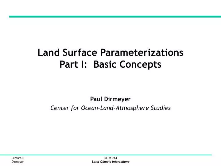
Land Surface Parameterizations Part I: Basic Concepts . Paul Dirmeyer Center for Ocean-Land-Atmosphere Studies. Parameterizations. pa·ram·e·ter·i·za·tion noun Etymology: New Latin, from para- + Greek metron measure

E N D
Land Surface ParameterizationsPart I: Basic Concepts Paul Dirmeyer Center for Ocean-Land-Atmosphere Studies CLIM 714 Land-Climate Interactions
Parameterizations • pa·ram·e·ter·i·za·tion • nounEtymology: New Latin, from para- + Greek metron measure • 1 a function or representation using empirical relationships or arbitrary constants whose value characterizes a member of a system (as a family of curves); also: a quantity (as a mean or variance) that describes a statistical population • 2: an approximation of any of a set of physical properties whose values determine the characteristics or behavior of something Land surface models are parameterizations of the large-scale behavior of the land surface. Whereas the laws of thermodynamics and fluid mechanics are well known and easily scalable (the basis of ocean and atmosphere models), the “physics” of the land surface is, by and large, complex, imperfectly understood, and not easily scalable. CLIM 714 Land-Climate Interactions
The Bucket Model The first attempt to model an interactive land surface in a GCM was only about 35 years ago: Manabe, S., 1969: Climate and the circulation, I. The atmospheric circulation and the hydrology of the earth's surface. Mon. Wea. Rev., 97, 739‑774. Evaporation was calculated by a simple linear relationship: where w is the soil wetness and b is a moisture availability factor that varies with soil moisture content. Typically b has a form like: CLIM 714 Land-Climate Interactions
The Bucket Model evaporation precipitation radiation Soil moisture content Land surface parameterization scheme (sub)surface runoff The soil water capacity of a bucket is typically 15 cm of water. Why 15? The assumption is that the active soil column is 1 m deep. Soil porosity is around 0.45, so that column can hold 45 cm of water at saturation. The first third is below the wilting point, and unavailable for evaporation. The middle third is available, across the range from “completely stressed” to “completely unstressed”. The last (wettest) third is above field capacity, where any additional precipitation runs off. So the bucket represents the middle third of 45 cm = 15 cm. Of course, this is all quite arbitrary. There is also the “leaky bucket” where runoff can occur below b = 1. CLIM 714 Land-Climate Interactions
Other Methods Whereas the bucket uses the “beta method”, there is an alternative empirical method called the “alpha method”: a is a function of soil wetness, e is the vapor pressure, es is the saturated vapor pressure at atmospheric temperature TC, e is the psychrometric constant, ps is surface atmopsheric pressure, r is the density of air, and ra is the aerodynamic resistance. There is also a “threshold method”: • Where Ecis the evaporative flux from the soil. The “alpha” and “beta” methods reduce to the threshold method with the appropriate choices of a and b: • a ~ exp(-y) with being the matric potential • b = 1 forEp < Ec and b = Ec/Ep for EpEc). CLIM 714 Land-Climate Interactions
Uncertainty Leads to Variety As an example of the many forms for expressing potential evaporation, the following appendix is from a paper by Fedderer et al (1996): Notice the various independent variables listed: temperature, humidity, wind speed, solar radiation, canopy radiative properties, roughness, cloud cover, atmospheric stability, even length of day. CLIM 714 Land-Climate Interactions
The Green Bucket • The simplest improvement one can make on the Bucket Model is to add a proxy of vegetation effects: This is how evaporation was calculated in the NCEP reanalysis model! CLIM 714 Land-Climate Interactions
Vertical Structure in the Soil • The next level of complexity is to include vertical structure (i.e., more than one layer) in the soil. The simplest approach is known as the “Force Restore” method. It is still used today in some LSSs for heat or moisture transfer, but it is considered primitive. • Heat (or moisture) flows down gradient: Where is the heat flux vector (only vertical in our case), k is the thermal conductivity of the medium (soil), and C is the heat capacity of the soil. Substituting for : CLIM 714 Land-Climate Interactions
Vertical Structure in the Soil In the force-restore formulation, it is assumed that conductivity does not vary with depth, so that the prediction equation for surface temperature simplifies to: The general solution for a parabolic PDE of this type is straightforward: j is the e-folding depth at the frequency w, where the vertical coordinate z is positive downwards from the surface. CLIM 714 Land-Climate Interactions
Vertical Structure in the Soil For a single forcing frequency w (omitting the subscript j ): So that This is typically applied to two main forcing frequencies: the diurnal cycle and the annual cycle. This gives us, two “layers”; a shallow layer that can be penetrated by the diurnal cycle, and a deeper layer that is affected by the annual cycle: The depths where these equations apply are a function of the heat capacity, conductivity and frequency of forcing. Often the heat capacity is made a function of soil wetness, so that the depths may vary in time as soil wetness changes. That makes this scheme very difficult to validate with measurements in the field!! And what if there are forcings at other frequencies?? CLIM 714 Land-Climate Interactions
Discrete Vertical Layers - Heat • Most LSSs have discrete vertical layers, increasing in thickness with depth. This last point is borne from the derivation of the Force-Restore method, which shows that small spatial variations (with strong vertical gradients) are necessarily damped out as they penetrate the soil, leaving larger, broader structures to penetrate further. Thus, vertical resolution must be highest near the surface, and can be much coarser at depth. • Going back to our diffusion equations (now strictly in the vertical): We no longer constrain k to be constant — it may vary with depth. Conductivity depends on soil texture, soil wetness and soil structure, and there are many different ways to estimate it (all based on some kind of curve-fit to laboratory measurements). C is a function of soil texture and wetness q: qs is the porosity of the soil. CLIM 714 Land-Climate Interactions
Discrete Vertical Layers - Water Turning to soil wetness, from Darcy’s law: Note the resemblance to the heat diffusion equation on the previous page. Now F is the vertical moisture flux. There are two forces at work in the vertical. One is the force of gravity pulling water down. The other is the down-gradient diffusion of water which may be either up or down, depending on the profile of soil moisture. The flux can be expressed as: Where k(q) is the hydraulic conductivity, and l(q) is the hydraulic diffusivity; both functions soil wetness. CLIM 714 Land-Climate Interactions
Conductivity and Diffusivity Substituting into the predictive equation, we get: There are many functional relationships, allempirical, to express k and l in terms of soil wetness. They allow reduction of the above predictive equation to a single unknown. Most common in land surface schemes is the “Clapp and Hornberger” relationship: This approach lends itself to discretization into layers of finite thickness: Wherei is the layer number (typically 3-10 layers), and i+1/2 refers to the interface between layersi and i+1. CLIM 714 Land-Climate Interactions
Relating l and k to Soil Moisture There are many alternatives to the Clapp & Hornberger approach. Some are tailored to fit special situations very accurately. Some try to fit a broad range of soils reasonably well. Clapp & Hornberger is a broad approach. Many hydrologists prefer the method of van Genuchten: There are many variations on these two main approaches, as well as others both empirical, and based on knowledge of soil particle and pore size distributions. CLIM 714 Land-Climate Interactions
Beyond the Unsaturated Zone Typically the layers of a discrete soil model are restricted to the first few meters below the surface. At the bottom of the lowest layer, drainage is assumed to go into base flow, never to return. However, some models account for the water table, its contribution to runoff, and its ability to return soil water to the surface. These are a function of the depth of the water table: The logarithmic term is called the topographic index, which is a function of the local slope b and the upstream area a. Models that use a topographic index to determine the depth of the water table use the “TOPmodel” concept. CLIM 714 Land-Climate Interactions
Simulating the Water Table One variant is the VIC (Variable Infiltration Capacity) model. The figure at right shows how the fraction of precipitation P that contributes to runoff (Qd) increases as soil moisture Wo increases. Herei is the infiltration capacity, As is the fraction of a grid cell for which the infiltration capacity is less thani, andB determines the shape of the infiltration curve: CLIM 714 Land-Climate Interactions
The Family Tree Two main original SVATS (Soil-Vegetation-Atmosphere Transfer Schemes): BATS (Biosphere Atmosphere Transfer Scheme; Dickinson et al 1986) and SiB (Simple Biosphere; Sellers et al. 1986). These were among the first to include the effects of vegetation, although still in a highly empirical way. BATS uses simple curve fits, based on observational data, to keep the model efficient while including a broad range of important processes. SiB is quasi-physical, and attempts to simulate vegetation processes more directly. The original SiB and its SiBlings are based on the idea that plant moisture stress regulates ET. The latest evolutions of both models have shifted to a more realistic approach, where ET controls are based on photosynthesis demands. Most LSSs in the world today derive in some way from these two models, either by inspiration, formulation, or direct use of portions of their code. CLIM 714 Land-Climate Interactions
Transpiration Formulations These are as varied as the potential evaporation formulations CLIM 714 Land-Climate Interactions
Vegetation Type vs. Plant Functional Type These terms are often used interchangeably. Plant Functional Type (PFT) is a term used more by ecologists, and is more accurate in describing how vegetation is classified in LSSs. Most schemes use a small number of plant functional types, usually fewer than ten. They are primarily based on characteristics of growth form (tree, shrub, grass), leaf form (broad leaf, needle leaf), leaf phenology (evergreen, deciduous), and leaf physiology (C3, C4). C3/C4 refers to the specific chemical process used to create sugar from water, CO2, and light (called the "photosynthetic pathway"). All plants do C3 photosynthesis. The C3 pathway, also called Photosynthetic Carbon Reduction, involves catalysis by an enzyme called "RUBISCO" (the most abundant protein on the planet). It evolved when CO2 was more abundant in the atmosphere, and O2 was rarer. RUBISCO. The problem with C3 is that RUBISCO can also catalyze reactions with O2 (called photorespiration) which does nothing to feed the plant. About 6 CO2 are fixed by RUBISCO for every 1 O2. "C3" comes from the fact that the first product of CO2 fixation is 3‑phospho‑glycerate, a 3-carbon compound. CLIM 714 Land-Climate Interactions
C3 & C4 Some plants (mostly grasses in warm regions) have evolved another pathway called C4. Plants with C4 achieve a lower rate of photorespiration than their pure C3 counterparts. They produce a 4-carbon compound ‑ oxaloacetic acid. In the C4 pathway, no O2 is fixed, so the process is more efficient. But it is also more temperature sensitive. CLIM 714 Land-Climate Interactions
Handling Vegetation Heterogeneity Some examples: BATS, SiB:“Big leaf” models with one vegetation type per grid LSM: Includes a few extra “hybrid” vegetation types to account for some common, simple vegetation combinations Mosaic: A number of defined homogeneous vegetation types tile each grid with fractions of each Sechiba: Like Mosaic, except fluxes are not blended at the surface, but at the top of the boundary layer CLIM 714 Land-Climate Interactions
Soil Heterogeneity Runoff: Infiltration: Many LSSs represent the transient and highly spatially variable nature of convective precipitation by assuming a sub-grid distribution of rain where most of the rain falls over a very small area. This enhances runoff. Also, soil texture may vary greatly over a distance of meters. Diffusivity and conductivity can vary by orders of magnitude over a grid box. Evaporation: Stressed (no evapotranspiration), unstressed (ET below the potential rate), and saturated (wetlands, rivers, etc.) (e.g., new model from Koster & Ducharne) CLIM 714 Land-Climate Interactions
CHASM (CHAmeleon Surface Model) Desborough (1999) developed an LSS which can can be operated in a variety of surface energy/water balance modes ranging from Manabe's simple bucket, up to a complex SVAT scheme. Comparison of modes of complexity of CHASM in four PILPS experiments: GCM-derived a) tropical forest and b) grassland sites from PILPS(1); c) Cabauw PILPS 2(b); d) HAPEX MOBILHY PILPS 2(a). Dots represent all of the participating PILPS models. CHASM modes from simplest to most complex: M69 (Manabe bucket), SIMP (has snow and baseflow); SIMP-A (has stability correction in flux terms); RS (includes a surface resistance at the value shown (s m-1)); SLAM (full SVAT scheme with canopy resistance and tiles a la Mosaic. CLIM 714 Land-Climate Interactions
Carbon • Leaf photosynthesis is limited by one of three things: • availability of light • maximum rate of the Rubisco enzyme process • Carbon compound export (C3) or PEP-Carboxylase limitation (C4) • The rate of carbon flux into the plant can be modeled in the same way as transpiration out of the plant — as a diffusive flux through the stomata, regulated by stomatal conductance. • When carbon is in the model, the CO2 gradients can also affect rc. The rate at which photosynthesis "fixes" carbon in the plant (converts from gaseous CO2 to sugars) affects the CO2 concentration in the leaf, and thus the flux rate: Thus, a carbon budget can be kept along with the water and energy budgets. These models can be used in ecology and global change studies. Fancier elements can be added, like nutrient (nitrogen) dependence, storage of carbon in the soil, etc. CLIM 714 Land-Climate Interactions
Choosing Parameters With a complex LSS, how does one choose all the parameters? Some are measured in the field, although it is necessary to extrapolate measurements for a few or one species to all members of a vegetation type. This leaves a great deal of uncertainty (and potentially inaccuracy) for simulations where a complete set of parameters are not available. And some parameters are not measurable. Another alternative is to calibrate the model at locations with observed fluxes (but not necessarily observed model parameters). This can be done by changing each parameter one-at-a-time. A better approach is to use a “multi-criteria” method where all parameters are tuned simultaneously to minimize errors across multiple measured variables. CLIM 714 Land-Climate Interactions
Optimal Approaches to Parameters One can remove almost all of the error from one variable this way, at the expense of errors in other variables. One cannot remove all the errors in all fluxes this way, because the LSS is not perfect, and does not include every process in the real world. It has been found that when models are tuned to minimize error in this way, complex schemes generally perform better than simple schemes, but the rate of improvement decays as complexity increases. CLIM 714 Land-Climate Interactions
What About Snow? • Snow is a complicating factor, as is freezing/thawing of soil. It is a lot easier to simulate land surface processes during the warm season than during the cold season. Snow affects absorption of solar radiation (high albedo), surface temperature (insulation), evaporation (availability of moisture). • Simple (e.g., original SiB): any snow is spread uniformly across the grid box. • Problem: albedo goes way up with the first snowflake. • Fractional coverage: snow coverage ramps up from 0 to some critical snow depth, to allow albedo to increase gradually. • Problem: a deep snowpack will have vertical gradients in temperature, density, and radiation penetration. • Multi-level snow model: Like a multi-level soil model. • What about vegetation and snow? • As snow accumulates, it covers low vegetation (e.g. grass). But snow remains under a canopy, and can be shaded or obscured (even under the branches of a deciduous canopy). This was not taken into account in most models until recently. This omission lead to a cold bias over snow in both the NCEP and ECMWF forecast models, and was diagnosed with the aid of data from remote sensing and the BOREAS field experiment. CLIM 714 Land-Climate Interactions
Other Heterogeneities Precipitation: Convective rainfall may be assumed to fall non-uniformly over a grid box. Most of the rain falls with high intensity over a fraction of the area. This means less precipitation infiltrates the soil, and more precipitation runs off than would happen with a steady, uniform rain. The parameterization of sub-grid precipitation allows for a more realistic surface water balance. Temperature: Aside from the mosaic tiling of surface cover types, the variation of temperature with elevation within a grid box may also be included. This can be very important in mountainous terrain. Orography can also be tied to sub-grid distributions of snow. Lakes/Wetlands: Open water from large rivers or lakes can be an important source of moisture fluxes and temperature moderation in certain conditions (e.g., arid regions, early winter (high latent and sensible heat flux), and spring (frozen water, reduced fluxes). Seasonal wetlands can also affect fluxes well into the dry season where monsoon seasonality is dominant. Some LSSs even include an explicit lake model (usually either a slab model, or a one-dimensional column model) CLIM 714 Land-Climate Interactions
Going 2-D It is important to recognize the difference between what happens at a point (e.g. a weather station, or a flux tower) and what happens over an area (as represented in a GCM). Most observational data are at individual points. Once a LSS is developed and calibrated in this way, it is often used in a GCM or regional model with little or no adjustment. This is especially true for hydrology: Imagine what happens as a small storm moves across the area of a grid box. At the point (j) there is no rain, then a brief period of heavy rain rates, then no rain. But averaged over the box, there is a nearly constant, light rain rate. A LSS calibrated to produce the proper partitioning of runoff and infiltration at a point, where rain rates are observed to fluctuate strongly, will produce little or no runoff when applied over large grids. Either the sub-grid distribution of rainfall must be parameterized, or the runoff parameterization must be reformulated to be appropriate at the larger spatial scale. CLIM 714 Land-Climate Interactions
Other Elements River routing: Most LSS do not concern themselves with water once it runs off. A river routing model is a means to couple the land to the ocean. More sophisticated routing models can simulate the interaction between the atmosphere and water bodies, seasonally inundated wetlands, and even floods. Human activity: The effects of human land use/abuse on the distribution of vegetation, or on its seasonal cycle (e.g. planting and harvesting, or grazing by livestock) can be simulated. Fire: Both natural and man-made fires affect both the land surface, and the atmosphere (aerosol production, radiative effects of smoke). These effects can be locally and regionally important. CLIM 714 Land-Climate Interactions
Other Elements Falls: Storms can cause treefalls or cropfalls over areas of importance at the mesoscale. The importance of this kind of land cover change on local climate is only beginning to be investigated. Species competition, global change: On longer time scales, the evolution of the biosphere as a whole can be modeled. This can be done statistically, by mapping vegetation types to particular climate zones and soil types, or dynamically by extending the carbon modeling to whole plant modeling (including growth, death, and competition between species or plant functional types). The first studies focused on the changes induced by ice-age fluctuations, where paleological evidence exists for the migration of vegetation. Emphasis is now shifting to prediction of responses to climate change and global warming. CLIM 714 Land-Climate Interactions
References Assouline, S., D. Tessier, and A. Bruand, 1998: A conceptual model of the soil water retension curve. Water Resour. Res., 34, 223‑231. Clapp, R., and G. Hornberger, 1978: Empirical equations for some soil hydrologic properties. Water Resour. Res., 14, 601‑604. Cosby, B. J., G. M. Hornberger, R. B. Clapp, and T. R. Ginn, 1984: A statistical exploration of the relationships of soil moisture characteristics to the physical properties of soils. Water Resour. Res., 20, 682‑690. Desborough, C. E., 1999: Surface energy balance complexity in GCM land surface models. Climate Dyn., 15, 389‑403. Dickinson, R. E., A. Henderson‑Sellers, and P. J. Kennedy, 1993: Biosphere‑Atmosphere Transfer Scheme (BATS) version 1E as coupled to the NCAR community climate model. Tech. Note NCAR/TN‑387+STR [Available from National Center for Atmospheric Research, Boulder, Colorado], 72 pp. Famiglietti, J. S., and E. F. Wood, 1994: Multiscale modeling of spatially variable water and energy balance processes. Water Resour. Res., 30, 3061‑3078. Federer, C. A., C. Vörösmarty, and B. Fekete, 1996: Intercomparison of methods for calculating potential evaporation in regional and global water balance models. Water Resour. Res., 32, 2315‑2321. Gupta, H. V., L. A. Bastidas, S. Sorooshian, W. J. Shuttleworth, and Z. L. Yang, 1999: Parameter estimation of a land surface scheme using multicriteria methods. J. Geophys. Res., 104, 19491‑19503. Lacis, A. A., and J. E. Hansen, 1974: A parameterization for the absorption of solar radiation in the Earth's atmosphere. J. Atmos. Sci., 31, 118‑133. Manabe, S., 1969: Climate and the circulation, I. The atmospheric circulation and the hydrology of the earth's surface. Mon. Wea. Rev., 97, 739‑774. Priestley, C. H. B., and R. J. Taylor, 1972: On the assessment of surface heat flux and evaporation using large‑scale parameters. Mon. Wea. Rev., 100, 81‑92. Sellers, P. J., Y. Mintz, Y. C. Sud, and A. Dalcher, 1986: A simple biosphere model (SiB) for use within general circulation models. J. Atmos. Sci., 43, 505‑531. van Genuchten, M. T., 1980: A closed‑form equation for predicting the hydraulic conductivity of unsaturated soils. Soil Sci. Soc. Am. J., 44, 892‑898. Wood, E. F., D. P. Lettenmaier, and V. G. Zartarian, 1992: A land‑surface hydrology parameterization with subgird scale variability for general circulation models. J. Geophys. Res., 97, 2717‑2728. CLIM 714 Land-Climate Interactions