Download
1 / 77
770 likes | 885 Views
IE-OR Seminar April 18, 2006. Evolutionary Algorithms in Addressing Contamination Threat Management in Civil Infrastructures Ranji S. Ranjithan Department of Civil Engineering, NCSU. Many security threat problems in civil infrastructure systems.

E N D
IE-OR SeminarApril 18, 2006 Evolutionary Algorithms in Addressing Contamination Threat Management in Civil Infrastructures Ranji S. Ranjithan Department of Civil Engineering, NCSU
Many security threat problems in civil infrastructure systems
Water distribution networks… • Solve for network hydraulics (i.e., pressure, flow) • Depends on • Water demand/usage • Properties of network components • Uncertainty/variability • Dynamic system • Solve for contamination transport • Depends on existing hydraulic conditions • Spatial/temporal variation • time series of contamination concentration
Water distribution networks… • Explain the contamination issues • Show animation
Why is this an important problem? • Potentially lethal and public health hazard • Cause short term chaos and long term issues • Diversionary action to cause service outage • Reduction in fire fighting capacity • Distract public & system managers
What needs to be done? • Determine • Location of the contaminant source(s) • Contamination release history • Identify threat management options • Sections of the network to be shut down • Flow controls to • Limit spread of contamination • Flush contamination
What needs to be done? • Determine • Location of the contaminant source(s) • Contamination release history • Identify threat management options • Sections of the network to be shut down • Flow controls to • Limit spread of contamination • Flush contamination
Example math formulation • Find: L(x,y), {Mt}, T0 • Minimize Prediction Error • ∑i,t || Cit(obs) – Cit(L(x,y), {Mt}, T0) || • where • L(x,y) – contamination source location (x,y) • Mt – contaminant mass loading at time t • T0 – contamination start time • Cit(obs) – observed concentration • Cit(L(x,y), {Mt}, T0) – concentration from system simulation model • i – observation (sensor) location • t – time of observation
Example math formulation • Find:L(x,y), {Mt}, T0 • Minimize Prediction Error • ∑i,t || Cit(obs) – Cit(L(x,y), {Mt}, T0) || • where • L(x,y) – contamination source location (x,y) • Mt – contaminant mass loading at time t • T0 – contamination start time • Cit(obs) – observed concentration • Cit(L(x,y), {Mt}, T0) – concentration from system simulation model • i – observation (sensor) location • t – time of observation • unsteady • nonlinear • uncertainty/error
Example math formulation • estimate solution state with currently available data • identify possible solutions that fit the data • assess confidence in current estimate of solution(s) • Find:L(x,y), {Mt}, T0 • Minimize Prediction Error • ∑i,t || Cit(obs) – Cit(L(x,y), {Mt}, T0) || • where • L(x,y) – contamination source location (x,y) • Mt – contaminant mass loading at time t • T0 – contamination start time • Cit(obs) – observed concentration • Cit(L(x,y), {Mt}, T0) – concentration from system simulation model • i – observation (sensor) location • t – time of observation
Interesting challenges • Non-unique solutions • Due to limited observations (in space & time) Resolve non-uniqueness • Incrementally adaptive search • Due to dynamically updated information stream Optimization under dynamic environments • Search under noisy conditions • Due to data errors & model uncertainty Optimization under uncertain environments
Interesting challenges • Non-unique solutions • Due to limited observations (in space & time) Resolve non-uniqueness • Incrementally adaptive search • Due to dynamically updated information stream Optimization under dynamic environments • Search under noisy conditions • Due to data errors & model uncertainty Optimization under uncertain environments
Evolutionary algorithm-based solution approach • Evolutionary algorithms (EAs) for numeric search • Genetic algorithms, evolution strategies • Key characteristics • Population-based probabilistic search • Directed “random” search • Conditional sampling of decision space • Updated statistics/likelihood values • Based on quality of prior solutions (samples)
Resolving non-uniqueness • Underlying premise • In addition to the “optimal” solution, identify other “good” solutions that fit the observations • Are there different solutions with similar performance in objective space? Search for alternative solutions [work conducted by Dr. Emily Zechman]
f(x) x Resolving non-uniqueness… • Search for alternative solutions
f(x) x Resolving non-uniqueness… • Search for different solutions that are far apart in decision space
Resolving non-uniqueness… • Effects of uncertainty f(x) x
Resolving non-uniqueness… • Search for solutions that are far apart in decision space and are within an objective threshold of best solution f(x) x
Resolving non-uniqueness…EAs for Generating Alternatives (EAGA) Create n sub populations Sub Pop 1 Sub Pop 2 . . . Evaluate obj function values Evaluate obj function values Best solution (X*, Z*) Feasible/Infeasible? Evaluate pop centroid (C1) in decision space Evaluate distance in decision space to other populations Selection (obj fn values) & EA operators Selection (feasibility, dist) & EA operators . . . Y N Y N STOP? STOP? Best Solutions
EAGA…Illustration using a test function • y = [(1 - 10x)*sin(11*x)]2 / [2.83*(10x)1.46]
EAGA…Illustration using a test function • y = [(1 - 10x)*sin(11*x)]2 / [2.83*(10x)1.46] • Generate 3 different solutions • Optimal and two alternatives • Within a 75% threshold of the optimal solution • Search using Evolution Strategies
EAGA…Illustration using a test function • y = [(1 - 10x)*sin(11*x)]2 / [2.83*(10x)1.46]
c t Contaminant source identification Groundwater contamination problem 1
Resolving non-uniqueness…Using EAGA 1 • Objective function: • minimize prediction error • EAGA settings: • four different solutions • evolution strategies • = 200, µ = 100 • 40 generations • subpopulation size 100 • 30 random trials • Decision Variables: • center of source (x, y) • size in x direction • size in y direction • concentration
Resolving non-uniqueness, using EAGA… Observations from Well 1 only
Resolving non-uniqueness, using EAGA… Observations from Well 1 only… Predictions At Well 1
Resolving non-uniqueness, using EAGA… Observations from Well 1 only… Predictions At Well 2
Resolving non-uniqueness, using EAGA… Observations from Wells 1 & 2
Resolving non-uniqueness, using EAGA… Observations from Wells 1 & 2… Predictions At Well 1
Resolving non-uniqueness, using EAGA… Observations from Wells 1 & 2… Predictions At Well 2
Interesting challenges • Non-unique solutions • Due to limited observations (in space & time) Resolve non-uniqueness • Incrementally adaptive search • Due to dynamically updated information stream Optimization under dynamic environments • Search under noisy conditions • Due to data errors & model uncertainty Optimization under uncertain environments
Dynamic optimization • Minimize Prediction Error • ∑i,t || Cit(obs) – Cit(L(x,y), {Mt}, T0) || • Cit(obs) – streaming data • Objective function is dynamically updated • Dynamically update estimate of source characteristics
Dynamic optimization… • Underlying premise • Predict solutions using available information at any time step • Search for a diverse set of solutions (EAGA) • Current solutions are good starting points for search in the next time step [work conducted by Ms. Li Liu]
Dynamic optimization… t = 1 f(x) x
Dynamic optimization… t = 2 f(x) x
Dynamic optimization… t = 3 f(x) x
Dynamic optimization…Adaptive Dynamic OPt Technique (ADOPT) • Set time step t=0 • Initialize sub-populations with random solutions • Construct obj function for time step t+1 • Apply EAGA to all sub-populations • Merge solutions to identify unique set of solutions • If t < Tmax, go to Step 3 • Record solution and stop
ADOPT…Illustration using a test function • Test function • where • B(x) is a time-invariant “basis” landscape • P is the function defining the shape of peak i • each of peak has its own time-varying parameters • h (height) • w (width) • p (shift) • 35 time steps
ADOPT…Results for the test function • 5-D case; avg error & std over all time steps, & 30 random trials
ADOPT…Illustration using a test function • 5-D case; avg error & std dev over all time steps
ADOPT…Contaminant source identification • Minimize Prediction Error • ∑i,t || Cit(obs) – Cit(L(x,y), {Mt}) || • Cit(obs) – streaming data • Objective function is dynamically updated • Is available information sufficient to be confident about current solution?