Download

1 / 51
510 likes | 540 Views
Markov Chain Monte Carlo Methods. By Marc Sobel. Exploring Monte Carlo. A biulding in the country of Monte Carlo:. Monte Carlo Goals.

E N D
Markov Chain Monte Carlo Methods By Marc Sobel
Exploring Monte Carlo • A biulding in the country of Monte Carlo:
Monte Carlo Goals • 1. Simulate observations from a density f(x) (having the property that it integrates to 1). We would like to visit sites in the proportion given by the density. • 2. Estimate expectations of the form: • by • With the x’s simulated under the density p.
Monte Carlo Theorem • The accuracy of the sampling sum depends only on the variance of ‘g’ and not on the dimensionality of the space. The Variance takes the form (where sigma-squared depends on g). • So what’s the problem. Suppose p(x) is known up to a constant of proportionality and • We could try to approximate the expectation by uniform sampling of the X’s over their range.
Monte Carlo Example • But in high dimensional spaces, this frequently doesn’t work well, since we have to pick an enormous number of uniform pts to get good accuracy: Suppose you wanted to map out and study the depths in a lake. Assuming the depth (viewed as a function of position) is quite complicated, uniform sampling will miss the important contours. Basically, the set of possible depth functions (i.e., the state space) is very large, so uniform sampling will tend to miss important parts of it.
Importance Sampling is (sometimes) the answer!! • Design a distribution h, from which we can sample, which captures the contours of ‘p’ properly. The estimate is then, • The quantities i=1,…,n are the • non-normalized weights attached to calculating the given expectation. • If they vary too little, the expectation tends to be inaccurate. If they vary too much, the sum may not converge.
Why Importance Sampling works • Why does importance sampling work?
Project • Could we assume h is a Gaussian? But suppose the underlying distribution is multimodal. Show that things go wrong when one variance is more than twice the others. Hint: Calculate the variance of the weights when the numerator p(x) is a mixture of gaussians and the denominator h is one gaussian from the mixture.
Importance Sampling (using independent variables) does not always work in high dimensions • Suppose x is the uniform distribution in a 1000 dimensional unit sphere. We approximate it by putting together 1000 independent gaussians each having variance σ2. The mean of the importance sampling distribution of r2=Σx2 is 1000σ2 with sd √2000σ2 . So, the typical weight will be: • Note that this means that weights with +√2000 will dominate all the rest.
An example of importance sampling Statisticians make frequent use of the t distribution with density in settings with large errors. ‘ν’ is the degrees of freedom, ‘θ’ is the mean, and ‘σ’ is the standard deviation.
Importance Sampling Example Can we use the normal to generate t distributions. Assume θ=0; σ=1; ν=4 degrees of freedom. Create standard normal rv’s z1,…,zn. Create (normalized weights) Give weights wi to zi (i=1,..,n). The resulting sample has a t distribution.
Matlab Code for importance sampling • zz= normrand(0,1,500,1); • w= tpdf(zz,4)./normpdf(zz); • ww = w/sum(w); • tt= randsample(zz,500,true,w)
Rejection Sampling • Our goal is to simulate from f. Instead we simulate from (a dominating distribution) Q. Q is dominating in the sense that there is a constant c with the property that cQ>f. For each simulated point xi, we also simulate a uniform variate ui between 0 and 1. If ui<f(xi)/cQ(xi) then we accept the point; otherwise we reject it.
Rejection Sampling • Why does rejection sampling work? Use Bayes theorem – a constant problem-solver:
Rejection Sampling:The Key • Say f is the target density, q is the simulating density, and c is the constant:
An Example of rejection sampling • We want to simulate a normal random variable truncated to be above 3. We use a dominating exponential distribution: • With constant c=2/[3(1-Φ(3))√2π]. So, we create • Exponential random variables Xi and uniforms Ui, rejecting when • Ui< φtrunc(Xi )/cΕΧΡ1.5(Xi).
Matlab code for rejection sampling in generating a truncated normal • num=0; • c=3/(2*sqrt(2*pi)); • for ii=1:1000 • zz=0; • while zz<3, • zz=exprnd(2/3); • end • w=normpdf(zz)/(c*exppdf(zz,2/3)); • if(rand<w) num=num+1; ss(num)=zz; end • end • ss
Truncated normal simulated by exponential: acceptance rate=20%
Problems with rejection sampling • If the constant ‘c’ is too large, (as will be the case in high dimensions) rejection sampling fails because the acceptance rate is so small. • If the contours of the ground truth distribution don’t correspond to those of the proposal distribution (e.g., one is multi and the other is unimodal), then rejection sampling fails to properly capture those contours. (Possible Project: Construct an example of this)
Rejection Sampling in High Dimensions • The ground truth space is 1000 dimensional (iid) gaussian space with component means 0 and standard deviation σP. If we use rejection sampling to simulate it using gaussians with component means 0 and standard deviations σQ =.99σP. Using the fact that, • We see that to use rejection sampling, we need to use c= 20,000. This means that the acceptance rate is about 1/20000=.00005.
Metropolis and the Hydrogen Bomb • Metropolis received his B.Sc. (1937) and Ph.D. (1941) degrees in experimental physics at the University of Chicago. Shortly afterwards, Robert Oppenheimer recruited him from Chicago, where he was at the time collaborating with Enrico Fermi and Edward Teller on the first nuclear reactors, to the Los Alamos National Laboratory. He arrived in the Los Alamos, on April 1943, as a member of the original staff of fifty scientists. After the World War II he returned to the faculty of the University of Chicago as an Assistant Professor. He came back to Los Alamos in 1948 to lead the group in the Theoretical (T) Division that designed and built the MANIAC I computer in 1952 and MANIAC II in 1957. (He chose the name MANIAC in the hope of stopping the rash of such acronyms for machine names, but may have, instead, only further stimulated such use.) From 1957 to 1965 he was Professor of Physics at the University of Chicago and was the founding Director of its Institute for Computer Research. In 1965 he returned to Los Alamos where he was made a Laboratory Senior Fellow in 1980. • Metropolis contributed several original ideas to mathematics and physics. Perhaps the most widely known is the Monte Carlo method. Also, in 1953 Metropolis co-authored the first paper on a technique that was central to the method known now as simulated annealing. He also developed an algorithm (the Metropolis algorithm or Metropolis-Hastings algorithm) for generating samples from the Boltzmann distribution, later generalized by W.K. Hastings.
Metropolis-Hastings to the rescue!! • We need to do ‘smart’ (rather than dumb) monte carlo. Smart monte carlo takes account of the past where importance and rejection sampling do not. For Metropolis Hastings we need a proposal density Q(xnew ,xcurrent) which tells us how to move from current point xcurrent to the new point. Suppose P is the ground truth density (from which we would like to sample). We simulate a point using the proposal distribution and ‘accept’ it only if it is ‘likely’ – not ‘more likely’. Basically, MH is a hill climbing algorithm.
Hill Climbing for Academics • You want to explore a hill. You are particularly interested in the hill’s terrain near the top. After each step, you analyze the terrain at that point. • Greedy algorithm: After each step. Propose a path which always goes up the hill. Note that you get stuck at local peaks where the only way to go is down. • Metropolis: At each step, propose a path; always take it if it is going up, but sometimes take it even if it is going down. In this way, you can break out of local peaks.
Good versus Evil!!! • Metropolis Hastings greedy algorithms
Formal Metropolis Hastings • Our goal is to visit sites in proportion to their posterior probability --- Metropolis only moves to a new position depending on its likelihood: the probability of moving is:
Metropolis Explanation The ratio measures the real Likelihood ratio but if it is very likely that we visit the new value xnew, then we have to discount it’s likelihood; we do this by using the factor,
Proof that Metropolis works • We show why it works. To do this, we show ‘the equation of balance’: • This shows that, • Therefore the resulting x’s are distributed according to the steady state distribution of the chain.
Proof (continued) • We show balance: • And this is the same with the other side of the equation, by symmetry.
Example: Simulating Multivariate Gaussian variables using independent Gaussians • Suppose we would like to simulate values from • We use the proposal: • Z’s are standard normals. The determinant is designed to correspond to the ground truth.
The move Probability • The move probability is: • So generate a vector using independent normals, then calculate the move probability, and move if it is realized, otherwise, don’t.
Devise a Metropolis Hastings algorithm to do rejection sampling when there is no dominating distributionavailable • Suppose we want to simulate from a complicated density f(x) and instead simulate from a density h(x) which does not dominate f (i.e., there is no c with the property f(x)<ch(x)). First, choose a c for f(x)<ch(x) for some x. Next, we calculate that,
Move probabilities calculated to satisfy balance • If x,y∈C={u: f(u)/ch(u)<1} α(y|x)=1 and α(x|y) [f(y)f(x)/cd]= [f(x)f(y)/cd], so α(x|y)=1. If x ∉ C, but y ∈ C. Then α(x|y) =1 because x has high f value. So, α(y|x) [f(x)f(y)/cd]= [f(y)h(x)/d] or α(y|x)=[ch(x)/f(x)]; If x∈C, but y∉C. Then α(x|y) =[ch(y)/f(y)];
Probmove continued • If x ∉ C, but y ∉ C, suppose α(x|y)=1; α(y|x) [f(x)h(y)/d]= [f(y)h(x)/d] or α(y|x)=[f(y)h(x)/h(y)f(x)]∧1 Example: Use this to simulate from a t distribution with 4 degrees of freedoms by simulation from a standard normal r.v. Constant c=1.2.
Explanation: Basic code. • Define the set C as: • Start with x. • Then if x,yεC, move to y. • If yεC but x not in C, move to y with probability, cφ(x)/t4(x). Else y=x. • If xεC but y not in C, move to y with probability, cφ(y)/t4(y). Else y=x. • If neither x nor y is in C, move to y with probability, min{t4(y)φ(x)/[φ(y)t4(x)],1}. Else y=x.
Matlab code for • % compute a t distribution using a normal • x=0; y=0; c=1.2; suc=0; • % construct 5000 variables • for ii=1:5000 • % simulate x,y and determine whether x,y are in C. • nx=normpdf(x,0,1); ny=normpdf(y,0,1); • tx=tpdf(x,4); ty=tpdf(y,4); • if(tx<1.2*nx) x1=1; • else • x1=0; • end • if(ty<1.2*ny) y1=1; • else • y1=0; • end • % distinguish move probabilities based on occupancy • if(x1==1 & y1==1) alph=1; end • if(x1==1 & y1==0) alph=(1.2*normpdf(y,0,1))/tpdf(y,4); end • if(x1==0 & y1==1) alph=(1.2*normpdf(x,0,1))/tpdf(x,4); end • if(x1==0 & y1==0) alph=(tpdf(y,4)*normpdf(x,0,1)/... • (tpdf(x,4)*normpdf(y,0,1))); end • if(rand<alph) tt(ii)=y; suc=suc+(1/5000); • else • tt(ii)=x; • end • x=tt(ii); • y=normrnd(0,1); ss(ii)=y; • end
T distribution with 4 degrees of freedom simulated from a normal versus normal histogram
Gibbs Sampling • Gibb’s sampling is a special case of Metropolis where we always move. For k dimensional data it is the composition of k MH algorithms; the i’th is: • α(x[1],…,x[i],y[i],x[i+1],…,x[n] |x)=δy[i],x[i]g(y[i]|x)
Gibbs Sampling Example Simulate a normal random variable truncated above 5. Add a variable z and define the joint distribution, g(x,z)=constant δx>5δ0≤z≤exp{-(x-μ)2/2σ2} The marginal distribution of x is normal with mean mu and variance sigma-squared truncated above 5. We apply Gibbs sampling by sampling x conditional on z and then z conditional on x.
Gibbs Sampling • (x|z)= {5,3+√-2σ2log(z)} • This comes from solving the equation, • z< exp{-(x-μ)2/2σ2}; x>5 • (z|x)={0,exp(-(x-μ)2/2σ2)} • This comes from fixing x and ‘solving for z’.
Matlab Code for truncated normal using Gibbs Sampling • Mulower is the truncation point, mu is the normal mean, and sigma is the normal sd. • function tnp=truncpos(mulower,mu,sigma) • z=normpdf(mulower,mu,sigma)*sigma*sqrt(2*pi)*.2; • if(z<.0000000001 & mulower<mu) tnp=mu; return; end • if(z<.0000000001 & mulower>mu) tnp=mulower; return; end • for ii=1:10000 • if(z>1) continue; end • tnp=unifrnd(mulower,mu+sqrt(-2*sigma^2*log(z))); • z=unifrnd(0,normpdf(tnp,mu,sigma)*sigma*sqrt(2*pi)); • end
Simulation of a normal random variable with mean 3 and variance 1 truncated to be above 5 (simulation of 500 values).
Example: Simulating Multivariate Gaussian variables using Gibbs Sampling • Suppose we would like to simulate values from • We use the proposal: basic code is: • Z’s are standard normals.
Definition of Simulated Annealing • Simulated annealing (SA) is a generic probabilisticmeta-algorithm for the global optimization problem, namely locating a good approximation to the global optimum of a given function in a large search space. It was independently presented by S. Kirkpatrick, C. D. Gelatt and M. P. Vecchi in 1983, and by V. Černý in 1985. It originated as a generalisation of a Monte Carlo method for examining the equations of state and frozen states of n-body systems, invented by N. Metropolis et al in 1953. • The name and inspiration come from annealing in metallurgy, a technique involving heating and controlled cooling of a material to increase the size of its crystals and reduce their defects. The heat causes the atoms to become unstuck from their initial positions (a local minimum of the internal energy) and wander randomly through states of higher energy; the slow cooling gives them more chances of finding configurations with lower internal energy than the initial one. • By analogy with this physical process, each step of the SA algorithm replaces the current solution by a random "nearby" solution; if the new solution is better, it is chosen, whereas if it is worse, it can still be chosen with a probability that depends on the difference between the corresponding function values and on a global parameter T (called the temperature), that is gradually decreased during the process. The dependency is such that the current solution changes almost randomly when T is large, but increasingly "downhill" as T goes to zero. The allowance for "uphill" moves saves the method from becoming stuck at local minima—which are the bane of greedier methods.
Simulated Annealing for Academics • You want to explore atomic phenomena at low energies by slowly freezing settings – fast freezing sometimes fails to show what’s happenning. • Metropolis: At each step, propose a path; always move if the new point is more likely, but sometimes take it even if it is less likely. In this way, you can break out of local peaks. • Simulated Annealing: Begin as above. Eventually, propose paths which (more and more) tends to move to points which are more likely and tends to never move to points which are less likely. Note that since this doesn’t happen for awhile, you avoid early local peaks.