Download

1 / 15
170 likes | 447 Views
An Analysis of Heat Conduction with Phase Change during the Solidification of Copper. Jessica Lyn Michalski 1 and Ernesto Gutierrez-Miravete 2 1 Hamilton Sundstrand 2 Rensselaer at Hartford COMSOL-09 . Scope. Use COMSOL to predict and visualize heat transfer including phase change

E N D
An Analysis of Heat Conduction with Phase Change during the Solidification of Copper Jessica Lyn Michalski1 and Ernesto Gutierrez-Miravete2 1Hamilton Sundstrand 2Rensselaer at Hartford COMSOL-09
Scope • Use COMSOL to predict and visualize heat transfer including phase change • Correlate known exact solutions for phase change to solutions created using COMSOL • Work carried out to fulfill requirements for the Masters degree in Mechanical Engineering at Rensselaer-Hartford.
Background • Phase changes occur in the production and manufacture of metals • Phase change, or moving boundary, problems are non-linear and few analytical solutions exist
Governing Equations Heat Equation (for Solid and Liquid Phases) dH/dt = div (k grad T) Thermal equilibrium at solid-liquid interface Stefan condition at the solid – liquid interface to define its location accounting for latent heat
Governing Equations Newmann obtained an exact solution for the solidification of a semi-infinite liquid region starting at a chilled wall Incorporation of the Stefan condition yields an equation for the solidification constant λ
Governing Equations The solidification constant is used to calculate the position of the solid – liquid interface, X, as a function of time In addition, it is also used to define the solid phase and liquid phase temperatures with respect to time and position
One – Dimensional AnalysisModel Creation • A one – dimensional model was created in COMSOL to model solidification of pure copper • Initial temperature = 1400 K • Temperature at Cold Wall = 400K • Thermal conductivity and specific heat were created first as constants and then as temperature dependent variables
One – Dimensional AnalysisModel Validation • Results from COMSOL were compared to the analytical solution and with the results of a finite difference solution • COMSOL results were obtained using a series of transient time step analysis options. Decreasing the time step increased the accuracy of the solution • The percent difference from the analytical solution was determined using the following equation:
Two – Dimensional AnalysisModel Creation • A two – dimensional model was also created in COMSOL • Initial temperature = 1400 K • Temperature at Cold Walls = 400 K • Two perpendicular sides assumed to be perfectly insulated • The two – dimensional system should behave similarly to the previous one – dimensional case along the lines x = L and y = L
Two – Dimensional AnalysisModel Validation • COMSOL results were created using one of the best options obtained in the one – dimensional analysis; the strict time step • Results from COMSOL two – dimensional analysis were compared to analytical solutions obtained for the previous, one – dimensional case in the x and y – directions • The percent difference from the analytical solution was determined using the following equation:
Conclusions • COMSOL shows promise as an easy to use tool for the creation of accurate representations of problems involving heat conduction with change of phase. • The introduction of two simple functions defining thermal conductivity and specific heat as functions of temperature readily allows for the incorporation of latent heat effects in a COMSOL conduction heat transfer model and makes possible accurate predictions of the solid-liquid interface location in 1D systems. • Additional work should be done to optimize this concept including correlating the results to actual test data, particularly for multi-dimensional systems.