Download
1 / 36
420 likes | 738 Views
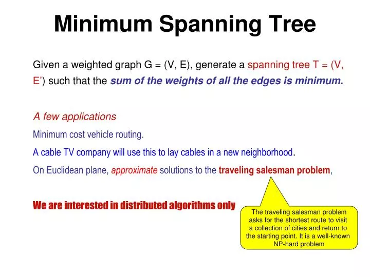
Minimum Spanning Tree. Given a weighted graph G = (V, E), generate a spanning tree T = (V, E’ ) such that the sum of the weights of all the edges is minimum. A few applications Minimum cost vehicle routing. A cable TV company will use this to lay cables in a new neighborhood .

E N D
Minimum Spanning Tree Given a weighted graph G = (V, E), generate a spanning tree T = (V, E’) such that the sum of the weights of all the edges is minimum. A few applications Minimum cost vehicle routing. A cable TV company will use this to lay cables in a new neighborhood. On Euclidean plane, approximate solutions to the traveling salesman problem, We are interested in distributed algorithms only The traveling salesman problem asks for the shortest route to visit a collection of cities and return to the starting point. It is a well-known NP-hard problem
Sequential algorithms for MST Review (1) Prim’s algorithm and (2) Kruskal’s algorithm(greedy algorithms) Theorem. If the weight of every edge is distinct, then the MST is unique.
GHS is a distributed version of Prim’s algorithm. Bottom-up approach. MST is recursively constructed by fragments joined by an edge of least cost. Gallagher-Humblet-Spira (GHS) Algorithm 3 7 5 Fragment Fragment
Challenges Challenge 1. How will the nodes in a given fragment identify the edge to be used to connect with a different fragment? A root node in each fragment is the root/coordinator
Challenges • Challenge 2. How will a node in T1 determine if a given edge connects to a node of a different tree T2 or the same tree T1? Why will node 0 choose the edge e with weight 8, and not the edge with weight 4? • Nodes in a fragment acquire the same name before augmentation.
Two main steps • Each fragment has a level. Initially each node is a fragment at level 0. • (MERGE) Two fragments at the same level L combine to form a fragment of level L+1 • (ABSORB) A fragment at level L is absorbed by another fragment at level L’ (L < L’). The new fragment has a level L’. (Each fragment in level L has at least 2L nodes)
To test if an edge is outgoing, each node sends a test message through a candidate edge. The receiving node may send accept or reject. Rootbroadcastsinitiate in its own fragment, collects the report from other nodes about eligible edges using a convergecast, and determines theleast weight outgoing edge. (Broadcast and Convergecast are two handy tools) Least weight outgoing edge test accept reject
Case 1. If name (i) = name (j) then send reject Case 2. If name (i) ≠ name (j) level (i) level (j) then send accept Case 3. If name (i) ≠ name (j) level (i) > level (j) then wait untillevel (j) = level (i) and then send accept/reject. WHY? (See note below) (Also note that levels can only increase). Q: Can fragments wait for ever and lead to a deadlock? Let i send test to j Accept of reject? Name = X reject test test Name = Y Note. It may be the case that the responding node belongs a different Fragment when it received the test message, but it is also trying to merge with the sending fragment.
The major steps repeat • Test edges as outgoing or not • Determine lwoe - it becomes a tree edge • Send join (or respond to join) • Update level & name & identify new coordinator/root until done
Classification of edges • Basic (initially all branches are basic) • Branch (all tree edges) • Rejected (not a tree edge) Branch and rejected are stable attributes (once tagged as rejected, it remains so for ever. The same thing holds for tree edges too.)
Merge The edge through which the join message is exchanged, changes its status to branch, and it becomes a tree edge. The new root broadcasts an (initiate, L+1, name) message to the nodes in its own fragment. Wrapping it up Example of merge initiate
Absorb T’ sends a join message to T, and receives an initiate message. This indicates that the fragment at level L has been absorbed by the other fragment at level L’. They collectively search for the lwoe. The edge through which the join message was sent, changes its status to branch. Wrapping it up initiate Example of absorb
Example 8 0 2 1 5 1 3 7 4 5 4 6 2 6 3 9
Example 8 merge merge 0 2 1 5 1 3 7 4 5 4 6 2 merge 6 3 9
Example 8 0 2 1 5 1 7 merge 3 4 5 4 6 absorb 2 6 3 9
Example absorb 8 0 2 1 5 1 7 3 4 5 4 6 2 6 3 9
Message complexity At least two messages (test + reject) must pass through each rejected edge. The upper bound is 2|E| messages. At each of the (max) log N levels, a node can receive at most (1) one initiate message and (2) one accept message (3) one join message (4) one test message not leading to a rejection, and (5) one changeroot message (to pick a new root of a fragment). So, the total number of messages has an upper bound of 2|E| + 5N log N
Leader Election Coordination Algorithms:
Leader Election Let G = (V,E) define the network topology. Each process i has a variable L(i) that defines the leader. The goal is to reach a configuration, where • i,j V i,j are non-faulty :: L(i) V and L(i) = L(j) and L(i) is non-faulty Often reduces to maxima (or minima) finding problem. (if we ignore the failure detection part)
Leader Election Difference between mutual exclusion & leader election The similarity is in the phrase “at most one process.” But, Failure is not an issue in mutual exclusion, a new leader is elected only after the current leader fails. No fairness is necessary - it is not necessary that every aspiring process has to become a leader.
Bully algorithm (Assumes that the topology is completely connected) 1. Send election message (I want to be the leader) to processes with larger id 2. Give up your bid if a process with larger id sends a reply message (means no, you cannot be the leader). In that case,wait for the leader message (I am the leader). Otherwise elect yourself the leader and send a leader message 3. If no reply is received, then elect yourself the leader, and broadcast a leader message. 4. If you receive a reply, but later don’t receive a leader message from a process of larger id (i.e the leader-elect has crashed), then re-initiate election by sending election message.
Bully algorithm Leader crashed election The worst-case message complexity =O(n3)(This is bad) 0 1 2 3 4 N-3 N-2 N-1 Node 0 sends N-1 election messages So, 0 starts all over again Node 1 sends N-2 election messages Node N-2 sends 1 election messages etc Finally, node N-2 will be elected leader, but before it sent the leader message, it crashed.
Chang-Roberts algorithm. Initially all initiator processes are red. Each initiator process i sends out token <i> {For each initiator i} dotoken <j> received j < i skip (do nothing) token <j> j > i send token <j>; color := black token <j> j = i L(i) := i {i becomes the leader} od {Non-initiators remain black, and act as routers} do token <j> received send <j> od Message complexity = O(n2). Why? What are the best and the worst cases? Maxima finding on a unidirectional ring The ids may not be nicely ordered like this
Franklin’s algorithm (round based) In each round, every process sends out probes (same as tokens) in both directions to its neighbors. Probes from higher numbered processes will knock the lower numbered processes out of competition. In each round, out of two neighbors, at least one must quit. So at least 1/2 of the current contenders will quit. Message complexity = O(n log n). Why? Bidirectional ring
Peterson’s algorithm initially i : color(i) =red, alias(i) =i {program for each round and for each red process} send alias; receive alias (N); if alias = alias (N) I am the leader alias ≠ alias (N) send alias(N); receive alias(NN); if alias(N) > max (alias, alias (NN)) alias:= alias (N) alias(N) < max (alias, alias (NN)) color := black fi fi {N(i) and NN(i) denote neighbor and neighbor’s neighbor of i}
Peterson’s algorithm Round-based. Finds maxima on a unidirectional ringusing O(n log n) messages. Uses an id and an alias for each process.
Synchronizers Synchronous algorithms (round-based, where processes execute actions in lock-step synchrony) are easer to deal with than asynchronous algorithms. In each round (or clock tick), a process (1) receives messages from neighbors, (2) performs local computation (3) sends messages to ≥ 0 neighbors A synchronizer is a protocol that enables synchronous algorithms to run on an asynchronous system. Synchronous algorithm synchronizer Asynchronous system
Synchronizers “Every message sent in clock tick k must be received by the neighbors in the clock tick k.” This is not automatic - some extra effort is needed. Consider a basic Asynchronous Bounded Delay (ABD) synchronizer Start tick 0 tick 0 tick 1 tick 2 tick 3 Start tick 0 Channel delays have an upper bound d Start tick 0 Each process will start the simulation of a new clock tick after2dtime units, where d is the maximum propagation delay of each channel
a-synchronizers What if the propagation delay is arbitrarily large but finite? The a-synchronizer can handle this. m ack m ack m Simulation of each clock tick ack Send and receive messages for the current tick. Send ack for each incoming message, and receive ack for each outgoing message Send a safe message to each neighbor after sending and receiving all ack messages (then follow steps 1-2-3-1-2-3- …)
Complexity of -synchronizer Message complexity M() Defined as the number of messages passed around the entire network for the simulation of each clock tick. M() = O(|E|) Time complexity T() Defined as the number of asynchronous rounds needed for the simulation of each clock tick. T() = 3 (since each process exchanges m, ack, safe)
Complexity of -synchronizer MA = MS + TS. M() TA = TS. T() MESSAGE complexity of the algorithm implemented on top of the asynchronous platform Time complexity of the original synchronous algorithm in rounds Message complexity of the original synchronous algorithm TIME complexity of the algorithm implemented on top of the asynchronous platform Time complexity of the original synchronous algorithm
The -synchronizer Form a spanning tree with any node as the root. The root initiates the simulation of each tick by sending message m(j) for each clock tick j. Each process responds with ack(j) and then with a safe(j) message along the tree edges (that represents the fact that the entire subtree under it is safe). When the root receives safe(j) from every child, it initiates the simulation of clock tick (j+1) using a next message. To compute the message complexity M(), note that in each simulated tick, there are m messages of the original algorithm, m acks, and (N-1)safe messages and (N-1) next messages along the tree edges. Time complexity T() = depth of the tree. For a balanced tree, this is O(log N)
Uses the best features of both and synchronizers. (What are these?)* The network is viewed as a tree of clusters. Each cluster has a cluster-head Within each cluster, -synchronizers are used, but for inter-cluster synchronization, -synchronizer is used Preprocessing overhead for cluster formation. The number and the size of the clusters is a crucial issue in reducing the message and time complexities -synchronizer Cluster head * -synch has lower time complexity, -synchronizers have lower message complexity
Example of application: Shortest path • Consider Synchronous Bellman-Ford: • O( n |E| ) messages, O(n) rounds • Asynchronous Bellman-Ford • Many corrections possible (exponential), due to message delays. • Message complexity exponential in n. • Time complexity exponential in n, counting message pileups. • Using (e.g.) Synchronizer α: • Behaves like Synchronous Bellman-Ford. • Avoids corrections due to message delays. • Still has corrections due to low-cost high-hop-count paths. • O( n |E| ) messages, O(n) time • Big improvement.