Download
1 / 18
180 likes | 355 Views
4.3 Differentiated products. Vertical differentiation: different qualities Horizontal differentiation: equal qualities, but consumers perceive relevant differences. Models: Love of variety : representative consumer prefers n varieties to n goods of the same variety.

E N D
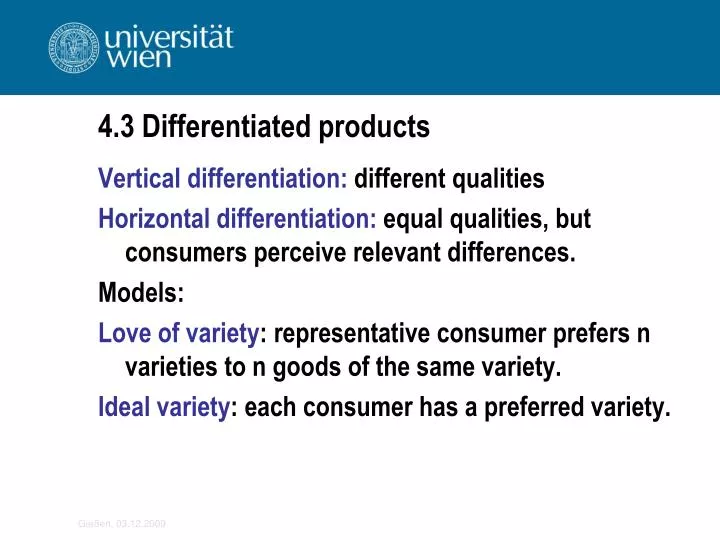
4.3 Differentiated products Vertical differentiation: different qualities Horizontal differentiation: equal qualities, but consumers perceive relevant differences. Models: Love of variety: representative consumer prefers n varieties to n goods of the same variety. Ideal variety: each consumer has a preferred variety.
4.3.1 Love of variety i = 1,…,N product varieties, N endogenous. Utility function u(c1,…,cN) which is strictly concave in ci implies “love of variety”. Partial Equilibrium Example 1: u(c) = v(ci), v’ > 0 > v”. The FOCs for maximizing utility obtained from the differentiated goods under the usual budget constraint are v‘(ci) = pi, i = 1,…,N (20)
v‘(ci) = pi, i = 1,…,N (20) Totally differentiating (20) and neglecting changes of (for large N) yields v“dci = dpi dci/dpi = /v“ < 0. Elasticity of demand for variety i: i = – [dci/dpi][pi/ci] = – v‘/civ“ > 0. Assumption: di/dci < 0.
Production: labor only factor, labor input: Li = F + axi ACi = wLi/xi = wF/xi + wa Equilibrium conditions under monopolistic competition (Chamberlin 1933): w = p/a Free entry zero-profit condition p = AC = wF/xi + wa p/w = F/Lc + a (21) Monopoly pricing MR = MC: p[1 – 1/] = wa p/w = a[/(1 – )] (22)
Equations (21) and (22) determine p/w and c. The number of firms (= varieties) is obtained from labor market clearing, hence L = Li = (F + axi) = N(F + ax) = N(F + aLc) N = 1/[F/L + ac]. Free trade between two identical countries: equivalent to a doubling of L: downward shift of ZZ-curve in figure 4.11: c (= quantity of each variety consumed per consumer) falls, but real wage (w/p) goes up, the number of varieties is increased, number of firms per country is reduced.
Predictions of the model: • Real wage is increased • Total number of varieties is increased • Individual consumption of each variety falls. • Number of firms per country falls. • Output per surviving firm is increased. Presumption: least efficient firms drop out. Two cost reducing effects: • Scale effect • Selection effect
Agrees with argument in favor of free trade made before trade agreements between U.S.A. and Canada: Domestic market too small for firms to operate at minimum efficient scale – free trade allows to expand exports, but not all firms in all countries can expand simultaneously – some firms will drop out, the remaining ones will produce more at lower average costs. • However, not supported by empirical evidence from U.S.A. and Canada free trade agreements: No scale effects, only selection effects
Example 2 • CES-utility function (Dixit & Stiglitz 1977): • Elasticity of substitution = > 1, which is also equal to for large N. Let := /( 1). The representative consumer solves
Implying the FOCs = marginal utility of income = v/I, i.e. partial derivative of indirect utility function w.r.t. income. The indirect utility function of a CES-function equals For n very large, effect of ci on and of pi on negligible.
Define the constant k as Substituting this into the FOC and re-arranging yields and thus = 1/[1 – ] = .
The markup of prices over MC is fixed, i.e. p/wa = /( − 1). (23) The profit equals = px – w(F + ax) = w[ax/( − 1) – F], and because of the zero profit condition output per firm equals x = ( − 1)F/a (24) The number of firms equals N = L/(F + ax). Thus, with free trade there is neither a scale effect nor a selection effect, but the number of varieties consumed is increased.
General equilibrium Assume there is also one homogeneous product, denoted as y, and total utility equals U(y,c) = y1-u(c). consumers devote a fraction of their income to buy differentiated products. Take the homogenous product as numeraire good, i.e. py = 1. Furthermore, factors of production are capital and labor. All goods have constant MCs, but the differentiated goods also have fixed costs F (e.g. F = rKx).
Integrated equilibrium with free entry: 1 = cy(w,r) = waLY + raKY (25) p = c(w,r,x) = waLX + raKX + rKX/x (26) p = [/( - 1)][waLX + raKX] (27) aLYy + aLXNx = L (28) aKYy + aLXNx + NKX = K (29) = pNx/[y + pNx] (30) Equations (25) and (26)are the zero profit conditions, (27) is implied by profit maximization, (28) and (29) are factor market clearing conditions, and (30) is market clearing for the differentiated goods.
Figure 4.12: FPE-set for differentiated goods (x) and one homogenous good (y).
Free entry: FPE-set analogous to perfect competition; inter-industrial trade AND intra-industrial trade. • Embodied factor services flows according to Heckscher-Ohlin model (factor abundance theory. • Fixed number of firms: FPE-set analogous to Cournot-oligopoly; country with larger number of monopolistic firms may import labor and capital services (paid for out of oligopoly rents).
The gravity equation Bilateral trade is directly proportional to the product of the countries‘ GDPs. Free trade equilibrium, all countries have identical prices, identical production functions and identical homothetic utility functions. C countries, N products, all prices normalized to equal one GDP = Yi = k yik , world GDP = Yw = Yi. sj = country j‘s share of world GDP = share of world expenditure.
Assuming that all countries are producing different varieties export of country i to country j of product k equals Xkij = sjyik. Summing over all products k yields Xij = Xkij= sjyik = sjYj = YjYi/Yw = sjsiYw = Xji. Summing the first and last term yields Xij + Xji = [2/Yw]YiYj. Explanation why trade grows faster than GDP.