Download
1 / 40
400 likes | 588 Views
Introduction to regression. Karen Bandeen -Roche, PhD Department of Biostatistics Johns Hopkins University. July 13, 2011. Introduction to Statistical Measurement and Modeling. Data motivation. Temperature modeling

E N D
Introduction to regression Karen Bandeen-Roche, PhD Department of Biostatistics Johns Hopkins University July 13, 2011 Introduction to Statistical Measurement and Modeling
Data motivation • Temperature modeling • Scientific question: Can we accurately and precisely model geographic variation in temperature? • Some related statistical questions: • How does temperature vary as a function of latitude and longitude (what is the “shape”)? • Does the temperature variation with latitude differ by longitude? Or vice versa? • Once we have a set of predictions: How accurate and precise are they?
United States temperature map http://green-enb150.blogspot.com/2011/01/isorhythmic-map-united-states-weather.html
Data examples • Boxing and neurological injury • Scientific question: Does amateur boxing lead to decline in neurological performance? • Some related statistical questions: • Is there a dose-response increase in the rate of cognitive decline with increased boxing exposure? • Is boxing-associated decline independent of initial cognition and age? • Is there a threshold of boxing that initiates harm?
Outline • Regression • Model / interpretation • Estimation / parameter inference • Direct / indirect effects • Nonlinear relationships / splines • Model checking • Precision of prediction
Regression • Studies the mean of an outcome or response variable “Y” as a function of predictor or covariate variables “X” • E[Y|X] • Note directionality: dependent Y independent X • Contrast to covariance, correlation: Cov(X,Y)=Cov(Y,X)
Regression • Purposes • Describing relationships between variables • Making inferences about relationships between variables • Predicting future outcomes • Investigating interplay among multiple variables
Regression Model • Y = systematic g(x) + random error • Y = E[Y|x] + ε(population model) • Yi = E[Y|xi] + εi, i = 1,…, n (sample from population) • Yi = fit(xi)+ ei (sample model) • This course: the linear regression model fit(X1,...,Xp;ß) = E[Y|X1,...,Xp] = ß0+ß1X1+...+ßpXp • Simple linear regression: One X yielding E[Y|X] = ß0+ß1X
Regression Model E[Y|X1,...,Xp] = ß0+ß1X1+...+ßpXp • Interpretation of β0: Mean response in subpopulation for whom all covariate values equal 0 • Interpretation of ßj: The difference in mean response comparing subpopulations whose xj value differs by one unit and values on other covariates do not differ
Modeling geographical variation:Latitude and Longitude http://www.enchantedlearning.com/usa/activity/latlong/
Regression – Matrix Specification • Notation: • n-vector v = (v1,...,vn)' (column), where “'” = “transpose” • nxp matrix A = (n rows, p columns) = [Aij], Aij = aij • E[Z] = (E[Z1],...,E[ZM])’ • Model: Y = Xß + ε • Y, ε = nx1 vector (n “records,” “people,” “units,” etc.) • X = nx(p+1) "design matrix“ • Columns: list ofones–codes the intercept–and then p Xs • ß= (p+1) vector (intercept and then coefficients β1,...,βp)
Estimation • Principle of least squares • Independently discovered by Gauss (1803) & Legendre (1805) • minimizes = • Resulting estimator: • “Fit” • = HY • “Residual” e= = • e = (I-H)Y ( )
Least squares fit - Intuition • Simple linear regression (SLR) • Fit=weighted average of slopes between each (xi,Yi) and : i.e.
Least squares fit - Intuition • Weight increases with distance of xi from sample mean of xs • LS line must go through : • Equally loaded springs attaching each point to line with fulcrum at • Multiple linear regression “projects” Y into the model space • = all linear combinations of columns of X
Why does LS yield a good estimator? • Need some preliminaries and assumptions • A preliminary – Variance of a random m-vector, z, is an (m x m) matrix, 1. Diagonal elements = variances: = Var(Zi) 2.(i, j) off-diagonal element = Cov(Zi, Zj) 3. = (symmetric) 4. is positive semi-definite: for any . 5. For an (n x m) matrix, A, Var
Why does LS yield a good estimator? • Assumptions – Random Part of the Model • A1: Linear model: • A2: Mean-0, exogenous errors: . • A3: Constant variance: has all diagonal entries = • A4: Random sampling: Errors are statistically independent. • A5: Probability distribution: is distributed as (~) multivariate normal (MVN)
Why does LS yield a good estimator? • Unbiasedness (“accuracy”): • Standard errors for beta: • To estimate: Will need estimate for • BLUE: LS produces the Best Linear Unbiased Estimator • SLR meaning: If is a competing linear unbiased estimator, then • MLR, matrix statement: is positive semidefinite i. e.g. for any choice of c0, …, cp
Inference on coefficients • We have • To assess: Will need estimate for • ei approximates • Estimate by ECDF variance of ei • Will justify “n-p” shortly • Estimated standard error of
Inference on coefficients • SE • 100 confidence interval for : • Hypothesis testing • versus • Test statistic: , • i.e., T follows a t distribution with n-p-1 degrees of freedom.
Direct and Indirect Associationsin Regression • Coefficients’ magnitude, interpretation may vary according to what other predictors are in the model. • Terminology • Consider two-covariate model: • = “direct association” of x1 with Y, controlling for x2 • The SLR coefficient in = “total association” of x1 with Y • The difference = “indirect association” through x2 and x1 with Y.
Direct and Indirect Associationsin Regression • The fitted total association of x1 with Y involves the fitted direct association and the regression of x2 on x1: • For SLR • where is the slope in the LS SLR of x2 on x1: = • Total, direct associations only equal if or • Generalizes to more than two covariates
Model Checking with Residuals • Two areas of concern • Widespread failure of assumptions A1-A5 • Isolated points: Potential to unduly influence fit • Model checking method • Fit full model, calculate and plot ei in various ways • Rationale: If model fits, ei mimics , so should have mean 0, equal variance, etc.
Model Checking with Residuals • Checking A1-A3: Scatterplots of residuals vs. (i) fitted values ; (ii) each continuous covariate xij, with reference line at y=0 • Good fit: flat, unpatterned cloud about reference line • A1-A2 violation: Curvilinear pattern about reference line • Influential points: Close to reference line at expense of overall shape • A3 violation: Tendency for degree of vertical “spread” about the reference line to vary systematically with or xij • Checking A5: Stem-and-leaf, ECDF-versus-normal plot
Nonlinear relationships: Curve fitting • Method 1: Polynomials • Replace by • Curve Method 2: “Splines” = piecewise polynomials • Feature 1: “order” = order of polynomials being joined • Feature 2: “knots” = where the polynomials are joined
How to fit splines • Linear spline with K knots at position k1, …, kK: where (x-k)+ = x-k if (x-k) > 0 and = 0 otherwise. • Spline of order M: where x – k0: =x. • To ensure a smooth curve, only include plus functions for the highest order terms
Spline interpretation, linear spline case • = Mean outcome in subpopulation with x=0 • = Mean Y vs. x slope on {x: x<k1} • = Amount by which mean Y vs. x slope on differs from slope on {x: x<k1} • = Amount by which mean Y vs. x slope on differs from slope on
Checking goodness of fit curveThe partial residual plot Larsen W, McCleary S. “The use of partial residual plots in regression analysis. Technometrics 1972; 14: 781-90. • Purpose: Assess degree to which a fitted curve describing association between Y and X matches the empirical shape of the association. • Basic idea • If there were no covariates except the one for which a curve is: being fit, we’d plot Y versus X and overlay with versus X. • Proposal: Subtract out contributions of other covariates
The partial residual plot - Method • Suppose model is , where • x2 = variable of interest & f(x2) = vector of terms involving x2, • represents “adjustment” for covariates other than x2 • Fit the whole model (e.g. get ); • Calculate partial residuals ; • Plot rp versus x2, overlaying with the plot of versus x2 • Another way to think about it: The partial residuals are + the overall model residuals.
United States temperature map http://green-enb150.blogspot.com/2011/01/isorhythmic-map-united-states-weather.html
Data motivation • Temperature modeling - Statistical questions: • How does temperature vary as a function of latitude and longitude (what is the “shape”)? - DONE • Does the temperature variation with latitude differ by longitude? Or vice versa? • Once we have a set of predictions: How accurate and precise are they?
Does the temperature variation with latitude differ by longitude? • Preliminary: Does temperature vary across latitude and longitude categories? • Usual device = dummy variables • Suppose the categorical covariate (X) has K categories • Choose one category (say, the Kth) as the “reference” • For other K-1 categories create new var. X1, …XK-1 with Xki = 1 if Xi = category k; 0 otherwise • Rather than include Xi in MLR, include Xi1, …, X-iK-1. • If more than one categorical variable, can create as many sets of dummy variables as necessary (one per variable)
Does the temperature variation with latitude differby longitude? • Formal wording: Is there interaction in the association of latitude and longitude with temperature? • Synonyms: effect modification, moderation • Covariates A and B interact if the magnitude of the association between A and Y varies across levels of B • i.e. B “modifies” or “moderates” the association between A & Y
Interaction Modeling • Interactions are typically coded as “main effects” + “interaction terms” • Example: Two categorical predictors (factors) • Model:
Interaction Modeling: Interpretations • = mean response at the “reference” factor level combination; = amount by which mean response at the second level of the first factor differs from the mean response at the first level of the first factor, among those at the first level of the second factor
Interaction Modeling: Interpretations = = amount by which the (difference in mean response across levels of the second factor) differs across levels of the first factor = amount by which the second factor’s effect varies over levels of the first factor.
How precise are our predictions? • A natural measure: ECDF Corr • “R-squared” = R2 • Temperatures example: R2 = 0.90 (spline model), R=0.95 • An extremely precise prediction (nearly a straight line) • Caution: This reflects precision for the SAME data used to build the model • Generally an overestimate of precision for predicting future data • Cross-validation needed: Evaluate fit in a separate sample
Main Points • Linear regression model • Random part: Errors distributed as independent, identically distributed N(0,σ2) • Systematic part: E[Y] = Xβ • Direct versus total effects • Differences in means • Nonlinear relationships: polynomials, splines • Interactions
Main Points • Estimation: Least squares • Unbiased • BLUE: Best linear unbiased estimator • Inference: Var( ) = σ2(X’X)-1 • Standard errors = square roots of diagonal elements • Testing, confidence intervals as in Lecture 2 • Model fit: Residual analysis • R2 estimates precision of predicting individual outcomes