Download
1 / 25
250 likes | 390 Views
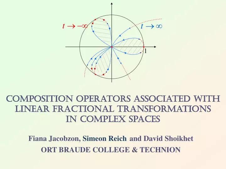
Composition Operators Associated with Linear Fractional Transformations in Complex Spaces. Fiana Jacobzon, Simeon Reich and David Shoikhet ORT BRAUDE COLLEGE & TECHNION. The Galton-Watson model Historical background.

E N D
Composition Operators Associated with Linear Fractional Transformations in Complex Spaces Fiana Jacobzon, Simeon Reichand David Shoikhet ORT BRAUDE COLLEGE & TECHNION
The Galton-Watson modelHistorical background One of the first applicable models of the complex dynamical systems on the unit disk arose more than a hundred years ago instudies of dynamics of stochastic branching processes. There was concern amongst the Victorians that aristocratic surnames were becoming extinct. Galton originally posed the question regarding the probability of such an event in the Educational Times of 1873, and the Reverend Henry William Watson replied with a solution. Together, they then wrote in 1874 paper entitled “On the probability of extinction of families. “
The Galton-Watson model Let us consider a process starting with a single particle which splits to an unknown number m of new identical particles in the first generation. Then in the next generation each one of mparticles splits to an unknown number of new identical particles and so on . . . I II This stochastic process is called the Galton-Watson branching process.
The Galton-Watson model I So we start at time t = 0 with a single particle (Z(0)=1) The first generation Z(1) is a random variable with distribution of probabilities Sincepm(1)is distribution of probabilities, then it generates function with Let ∆ be the open unit disk in C. Obviously,F:∆→∆ is an analytic function.
The Galton-Watson model I II The question is: What is the distribution of probabilities of a random variable Z(t) in the t-th generation? In other words, what is the probability p(n)k that after t = n generation the number of particles will be k?
The Galton-Watson model I II The question is very complicated because we do not know the situation in the previous generations.
then • It turns out, that if isn-iterateofF, i.e., F3(0) F2(0) F4(0) F5(0) F1(0) 0 The Galton-Watson model • So one can define the needed distribution of probabilities as • the coefficients of Taylor extension ofF(n) p It can be shown that there exists the limit which is called the extinction probability of the branching process.
One parameter semigroups of analytic mappings Let ∆ be the open unit disk in the complex planeC, andF : ∆ → ∆bean analytic function in ∆ with values in∆. In this case one says thatFis aself-mapping of the unit disk∆. Consider the familyS={F0, F1, F2,...}of iterates ofF i.e., F0= I, F1=F, F2= FoF=F2, ... In other words, F0(z)=z, F1(z)=F(z), F2(z)=F(F(z)),… The pair (∆, S ) is calledadiscrete dynamic system.
y x 1 One parameter semigroups of analytic mappings For anyz Є∆we can construct the sequence{Fn(z)}nЄN(N={0,1,2…}) of points in∆. F1(z) F2(z) F5(z) {F(n)(z)}nЄN F3(z) z F4(z) ∆
The iteration problem Consider a family of the functions: S={F0, F1, F2,...}such that F0= I, F1=F, F2=F(2),... , Fn= F(n),... Find F(n)explicitly for alln = 1,2,3,… This problem can be solved by using the so-called Koenigs embedding process. To do this we first should find a continuous functionu (t , z) = Ft (z)in parameter t , such that • F1= F • Ftpreserves iteration property for allt ≥ 0 A family of functions that satisfies both these properties is called a continuous semigroup.
F1¾(z) F1(z) F2(z) F5(z) F½(z) F3(z) z F4(z) F4⅔(z) Continuous semigroups of analytic functions A family S={Ft}t≥0is called a one-parameter continuous semigroup (flow) in ∆ if For integertwe get by property (i) than F1 isF, thanF2is F(2)and The pair (∆,S) is called a continuous dynamic system.
F3(0) F2(0) F4(0) F5(0) F1(0) 0 Embedding problem A classical problem of analysis is given an analytic self-mapping F ofthe open unit disk ∆, to find a continuous semigroup S={Ft}t≥0 in ∆such that F1=F. If such a semigroup exists then F is said to be embeddable. In general there are those self-mappings which are not embeddable. So, the problem becomes: describe the class of self-mappings which are embeddable.
Continuous semigroups of Linear Fractional mappings The interest of the Galton-Watson model has increased because of connections with chemical and nuclear chain reactions, the theory of cosmic radiation, the dynamics of disease outbreaks in their generations of spread. Most of those discreteapplications based on semigroups produced from the so-called Linear Fractional Mappings(LFM), i.e., analytic functions in the complex plane of the form:
Coefficients Problem • Find the conditions on the coefficients of an LFM which • ensure that it preserves the open disk Δ. Another important problem is finding conditions on a self-mapping F which ensure that it can be embedded into a continuous semigroup. In particular, for LFM this problem can be reformulated as follows: • Find the condition on the coefficients of LFM which ensure the • existence of a continuous semigroupS={Ft}t≥0 in ∆, • such thatF1=F.
F3(z) F2(z) F4(z) F5(z) F1(z) z Solution The important key to solve our problem is the asymptotic behavior of the semigroup in both discrete and continuous cases. It described in the well-known Theorem of Denjoy and Wolff. Theorem (Denjoy-Wolff, 1926) Let ∆ be the open unit disk in the complex plane C. If an analytic self-mapping F is not an elliptic automorhpism of ∆, then there is an unique point τin ∆U∂∆such that the iterates {F(n)(z)}nЄNconverge to τuniformlyon compact subsets of ∆. The point τis called the Denjoy –Wolff point of the semigroup and it is a common fixed point of {F(n)(z)}nЄN. If, in particular, F is a producing function of a Galton-Watson branching process, then τ is exactly the extinction probability of this process. E. Berkson and H. Porta (1981) established a continuous analog of Denjoy-Wolff theorem for continuous semigroups of analytic self-mapping of ∆. τ
Examples 1. Dilation case (rotation + shrinking): - the common fixed point (a)Re c = 0 (group of rotations) (b)Re c ≠ 0
- the common DW point Examples 2. Hyperbolic case (shrinking the disk to a point):
- the common DW point Examples 3. Parabolic case :
τєΔ • dilation τє∂∆, 0<F’ (τ)<1 • hyperbolic τє∂∆, F’ (τ)=1 • parabolic Classification Since the class of analytic self-mappings comprises three subclasses: with different features and properties, we consider these classes separately.
Proposition 1 (Elin, Reich and Shoikhet, 2001) Let F : Ĉ → Ĉbe an LFM of the form The following assertions hold: • F analytic self-mapping of Δ if and only if | a |+| c | ≤ 1; • If i.holds and a ≠ 0 then F is embeddable into continuous semigroup of analytic self mappings ofΔif and only if In particular, if a єR, then F is alwaysembeddable into a continuous semigroup of analytic self-mappings of Δ. Results Dilation case
Proposition 2 Let F : Ĉ → Ĉbe an LFM of the form with F (1) = 1 and 0<F’ (1) <1. The following assertion are equivalent: • |c / b| ≤ 1andc ≠ -b; • F analytic self-mapping of Δ of hyperbolic type; • F is embeddable into continuous semigroup of analytic self-mappings ofΔ. Results Hyperbolic case
Proposition 3 Let F : Ĉ → Ĉbe an LFM of the form with F (1) = 1 and F’ (1) =1. The following assertion are equivalent: • Re(d / c) ≤ -1andd ≠ -c; • F analytic self-mapping of Δ of parabolic type; • F is embeddable into continuous semigroup of analytic self-mappings ofΔ. Results Parabolic case
with F (τ) = τand0<|F’ (τ)| <1. The Method Our method of proof based on the so-called Koenigs function, which is a powerful tool to solve also many other problems as well as computational problems. Namely, consider for example an LFM of dilation or hyperbolic case, that is It was proven by Koenigs and Valiron that there exist a solution of the following functional equation of Shcroeder: h ( F(z)) = λh(z), where λ = F’ (τ) Thus, F can be represented in the form F(z) = h-1 ( λh(z)), where λ = F’ (τ) Then for all t ≥ 0 we can write Ft as Ft(z) = h-1 ( λth(z)), where λ = F’ (τ)
Let us consider an LFM of dilation type so Example The Koenigs function associated with F is Thus, F can be represented in the form F(z) = h-1 ( λh(z)), whereλ = F’ (τ) = ½, henceFt(z) = h-1 ( λt h(z)). Direct calculations show: In particular, substituting here t = n, we get explicitly all iterates F(n)=Fn
Thank you I II