Chap. 1 Systems of Linear Equations

1. Chap. 1Systems of Linear Equations 1.1 Introduction to Systems of Linear Equations 1.2 Gaussian Elimination and Gauss-Jordan Elimination 1.3 Applications of Systems of Linear Equations

2. Chapter Objectives • Recognize, graph, and solve a system of linear equations in n variables. • Use back substitution to solve a system of linear equations. • Determine whether a system of linear equations is consistent or inconsistent. • Determine if a matrix is in row-echelon form or reduced row-echelon form. • Use element row operations with back substitution to solve a system in row-echelon form. • Use elimination to rewrite a system in row echelon form. Chapter 1

3. Chapter Objective (cont.) • Write an augmented or coefficient matrix from a system of linear equation, or translate a matrix into a system of linear equations. • Solve a system of linear equations using Gaussian eliminationwith back-substitution. • Solve a homogeneous system of linear equations. • Set up and solve a system of linear equations to fit a polynomial function to a set of data points, as well as to represent a network. Chapter 1

4. 1.1 Introduction Linear Equations in n Variables • A linear equations in n variablesx1, x2, …, xn has the form: a1x1 + a2x2 + … + anxn = b • Coefficients: a1, a2, …, an  real number • Constant term: b  real number • Leading Coefficient: a1 • Leading Variable: x1 • Linear equations have noproducts or roots of variables and no variables involved in trigonometric, exponential or logarithmic functions. • Variables appear only to the first power. Chapter 1

5. Section 1-1 True? Example 1 • Linear Equations: • Nonlinear Equations: Product of variables involved in exponential involved in trigonometric Not the first power Chapter 1

6. Section 1-1 Example 2 Parametric Representation of a Solution Set • Solve the linear equation x1 + 2x2 = 4 Sol: x1 = 4  2x2 Variable x2 is free (it can take on anyreal value). Variable x1 is not free (its value depends on the value of x2). By letting x2 = t (t: the third variable, parameter), you can represent the solution set as • 參數個數=變數個數 方程式列數 Chapter 1

7. Section 1-1 Example 3 Parametric Representation of a Solution Set • Solve the linear equation 3x + 2y z = 3 Sol: Choosing y and z to be the free variables  Letting y = s and z = t, you obtain the parametric representation Infinite number of solutions Chapter 1

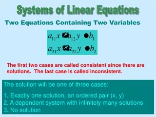
8. Section 1-1 Systems of Linear Equations • A system of m linear equations in n variables is a set of m equations, each of which is linear in the same n variables: • The double-subscript notation indicates that aij is the coefficient of xj in the ith equation. • A system of linear equations has exactly one solution, an infinite number of solutions, or no solution. • A system of linear equations is called consistent if it has at least one solution and inconsistent if it has no solution. Chapter 1

9. Section 1-1 y y x x y x Example 4 Systems of two equations in two variables • Solve the following systems of linear equations, and graph each system as a pair of straight lines. Two intersecting lines Two coincident lines Two parallel lines Chapter 1

10. Section 1-1 Solving a system of linear equations • Row-echelon form: it follows a stair-step pattern and has leading coefficient of 1. • Using back-substitution to solve a system in row-echelon form. • Example 6. 1. From Eq. 3 you already know the value of z. 2. To solve for y, substitute z = 2 into Eq. 2 to obtain y = 1. 3. Substitute z = 2 and y = 1 into Eq. 1 to obtain x = 1. Chapter 1

11. Section 1-1 Equivalent Systems • Two systems of linear equations are called equivalent if they have precisely the same solution set. • Each of the following operations on a system of linear equations produces an equivalentsystem. • 1. Interchange two equations. • 2. Multiply an equation by a nonzero constant. • 3. Add a multiple of an equationtoanother equation. • Gaussian elimination: Rewriting a system of linear equations in row-echelon form usually involves a chain of equivalent systems, each of each is obtained by using one of the three basic operations. Chapter 1

12. Section 1-1 Example 7 A system with exactly one solution • Solve the system Adding the second equation to the third equation produces a new third equation. Adding the first equation to the second produces a new second equation. Adding –2 times the first equation to the third equation produces a new third equation. (2)  (1/2) The solution isx = 1, y = 1, and z = 2. Chapter 1

13. Section 1-1 Example 8 (2) An Inconsistent System • Solve the system Adding –1 times the 2nd equation to the 3rd produces a new 3rd equation. Adding –1 times the first equation to the third produces a new third equation. Adding –2 times the first equation to the second produces a new second equation. (1) (1) Because the third “equation” is a false statement, this system has no solution. Moreover, because this system is equivalent to the original system, you can conclude that the original system also has no system. Chapter 1

14. Section 1-1 Example 9 A system with an infinite number of solutions • Solve the system Adding –3 times the 2nd equation to the 3rd produces a new 3rd equation. Adding the first equation to the third produces a new third equation. The first two equations are interchanged. (3) unnecessary Let x3 = t, t R Chapter 1

15. 1.2 Gaussain Elimination and Gauss-Jordan Elimination • Definition: Matrix If m and n are positive integers, then an mn matrix is a rectangular array in which each entry, aij, of the matrix is a number. • An mn matrix has mrows (horizontal lines) and ncolumns(vertical lines). • The entry aij is located in the ith row and the jth column. • A matrix with m rows and n columns (an mn matrix) is said to be ofsizemn. • If m = n, the matrix is called square of ordern. • For a square matrix, the entries a11, a22, a33, … are called the main diagonal entries. Chapter 1

16. Section 1-2 Augmented/Coefficient Matrix • The matrix derived from the coefficients and constant terms of a system of linear equations is called the augmented matrix of the system. • The matrix containing only the coefficients of the system is called the coefficient matrix of the system. • System Augmented MatrixCoefficient Matrix const. y z x Chapter 1

17. Section 1-2 Elementary Row Operations • Interchange two rows. • Multiply a row by a nonzero constant. • Add a multiple of a row to another row. Two matrices are said to be row-equivalent if one can be obtained from the other by a finite sequence of elementary row operations. Chapter 1

18. Section 1-2 Example 3 • Using Elementary Row Operation to Solve a System Linear System Associated Augmented matrix R2+R1R2 R3+(2)R1R3 R3+R2R3 (2) 0.5R3R3 0.5 Chapter 1

19. Section 1-2 Row-Echelon Form of a Matrix A matrix in row-echelon form has the following properties. • All rows consisting entirely of zeros occur at the bottom of the matrix. • For each row that does not consist entirely of zeros, the first nonzero entry is 1 (called a leading 1). • For two successive (nonzero) rows, the leading 1 in the higher row is father to the left than the leading 1 in the lower row. Remark: A matrix in row-echelon form is in reduced row-echelon form if every column that has a leading 1 has zeros in every position above and below its leading 1. Chapter 1

20. Section 1-2 Example 4 • In row-echelon form • Not in row-echelon form Chapter 1

21. Section 1-2 Gaussian Elimination withBack-Substitution • Write the augmented matrix of the system of linear equations. • Use elementary row operations to rewrite the augmented matrix in row-echelon form. • Write the system of linear equations corresponding to the matrix in row-echelon form, and use back-substitution to find the solution. Chapter 1

22. Section 1-2 (2) Example 5 A system with exactly one solution • Solve the system  6 Chapter 1

23. Section 1-2 (1) (2) (3) Example 6 A system with no solution • Solve the system 0 = 2 … ???The original system of linear equationsis inconsistent. Chapter 1

24. Section 1-2 (9) (3) Gauss-Jordan Elimination • Continues the reduction process until a reduced row-echelon form is obtained. • Example 7:Use Gauss-Jordan elimination to solve the system In Ex. 3  2 Chapter 1

25. Section 1-2 Example 8 • A System with an Infinite Number of Solutions Solve the system of linear equations Let x3 = t, t R Chapter 1

26. Section 1-2 Homogeneous Systems of Linear Equations Each of the constant terms is zero. • A homogeneous system must have at least one solution. • Trivial (obvious) solution: all variables in a homogeneous system have the value zero, then each of the equation must be satisfied. Chapter 1

27. Section 1-2 Example 9 • Solve the system of linear equations Let x3 = t, t R Chapter 1

28. Section 1-2 Theorem 1.1 The Number of Solutions of a Homogeneous System • Every homogeneous system of linear equations is consistent. Moreover, if the system has fewer equations than variables, then it must have an infinite number of solutions. Chapter 1

29. 1.3 Applications of Systems of Linear Equations • Polynomial Curve Fittingfit a polynomial function toa set of data points in the plane. • n points: • Polynomial function: • Network Analysisfocus on networks and Kirchhof’s Laws for electricity. Chapter 1

30. Section 1-3 Network Analysis • Networks composed of branches andjunctions are used as models in the fields as diverse as economics, traffic analysis, and electrical engineering. • The total flowinto a junction is equal to the total flow out of the junction. • Example. Chapter 1

31. Section 1-3      Example 5 Chapter 1

32. Section 1-3 Kirchhoff’s Laws • All the current flowing into a junction mustflow out of it. (KCL) • The sum of the products IR (I is the current and R is the resistance) around a closed pathis equal tothe total voltage in the path. (KVL) • A closed path is a sequence of branches such that the beginning point of the first branchcoincides withthe end point of the last branch. Chapter 1

33. Section 1-3 Example 6  or : Path 1: Path 2: Chapter 1

34. Section 1-3 Example 7 See pp. 37-38 in the textbook Chapter 1