Download
1 / 89
910 likes | 1.08k Views
CE 510 Hazardous Waste Engineering . Department of Civil Engineering Southern Illinois University Carbondale Instructor: Jemil Yesuf Dr . L.R. Chevalier. Lecture Series 8: Contaminant Release and Transport from Source. Course Goals.

E N D
CE 510Hazardous Waste Engineering Department of Civil Engineering Southern Illinois University Carbondale Instructor: Jemil Yesuf Dr. L.R. Chevalier Lecture Series 8: Contaminant Release and Transport from Source
Course Goals • Review the history and impact of environmental laws in the United States • Understand the terminology, nomenclature, and significance of properties of hazardous wastes and hazardous materials • Develop strategies to find information of nomenclature, transport and behavior, and toxicity for hazardous compounds • Elucidate procedures for describing, assessing, and sampling hazardous wastes at industrial facilities and contaminated sites • Predict the behavior of hazardous chemicals in surface impoundments, soils, groundwater and treatment systems • Assess the toxicity and risk associated with exposure to hazardous chemicals • Apply scientific principles and process designs of hazardous wastes management, remediation and treatment
Dispersion Of Air Pollutants • Focus on a basic point source Gaussian dispersion model • Assumptions: • Atmospheric stability is uniform • Turbulent diffusion is a random activity • Dilution in both the horizontal and vertical direction can be described by Gaussian or normal equations
Dispersion Of Air Pollutants • Assumptions (continued) • Contaminated gas stream is released into the atmosphere at a distance above the ground equal to the physical stack height plus the plume rise • Degree of dilution of the effluent plume is inversely proportional to the wind speed • Pollutant reaching the ground level is totally reflected back into the atmosphere like a beam of light striking a mirror at an angle ( image source)
Instantaneous Plume Boundary H h Time Averaged Plume Envelope
Gaussian Plume Model Eqn. 8.22 (Textbook) where: C (x,y,0,H) = downwind conc. at ground level(z=0), g/m3 Q = emission rate of pollutants, g/s sy, sz = plume standard deviation, m u = wind speed, m/s x,y,z and H = distance, m
Effective Stack Height The value for the effective stack height, H, is the sum of the physical stack height, h, and the plume rise DH. DH may be computed from Holland’s formula (J.Z. Holland, 1953, A Meteorological Survey of the Oak Ridge Area, U.S. Atomic Energy Commission Report No. ORO-99, Washington D.C., U.S. Government Printing Office)
Plume Rise where vs = stack velocity, m/s d = stack diameter, m u = wind speed, m/s P = pressure, kPa Ts = stack temperature, K Ta= air temperature, K
Gaussian Plume Model (see Table 8.1) p. 416
Gaussian Plume Model Need to evaluate these terms, which are the standard deviations of the plume
Gaussian Plume Model Martin, D.O., 1976. Comment on “The Change of Concentration Standard Deviation with Distance”, J. Air Pollut. Control Assoc., 26:145-147. sy = ax0.894 sz = cxd + f where x is the distance downwind, expressed in km, s is in m, and a,c,d, and f are constants found in the following table: NOTE: Alternatives are graphs 8.10 and 8.11
Example Consider the emission of SO2 from a coal fired power plant, at a rate of 1,500 g/s. The wind speed is 4.0 m/s on a sunny afternoon. What is the centerline concentration of SO2 3 km downwind (Note: centerline implies y=0). Stack parameters: Height = 130 m Diameter = 1.5 m Exit velocity = 12 m/s Temperature = 320°C (593° K) Atmospheric conditions: P=100 kPa T=25° C (298° K) Strategy
Strategy • Determine the effective stack height • D h • H = Dh + h • Determine stability class • Estimate sy and sz • Apply governing equation
Equations sy = ax0.894 sz = cxd + f
Solution H = effective stack height = h + DH = 130 m + 15.4 m = 145.4 m
Solution Atmospheric stability class: Class B sy = ax0.894 = 156(3)0.894 = 416.6 m sz = cxd + f = 108.2(3)1.098 + 2 = 363.5 m
Solution ... end of problem
Example Simplify the Gaussian dispersion model to describe a ground level source with no thermal or momentum flux, which is the typical release that occurs at a hazardous waste sites. In this situation, the effective plume rise, H, is essentially 0.
Puff Models • Instantaneous one-time release of material • Ground level where C is the concentration at (x,y,z,t) in mg/m3 Q’m is the mass of contaminant released (mg)
Puff Models For the plume dimensions (i.e. s) we will need to refer to Figures 8.8 and 8.9.
Example A hazardous waste spill has occurred, releasing 10 kg of TCE into the air. If the spill was at night under mostly overcast skies, and the wind velocity was 7 m/s in the x-direction, estimate the TCE concentration 0.5 km downgradient. Similar to Example 8.2. Instead of evaluating the spill at 0.5 km, evaluate the spill at 1 km. Compare s values as well as final value. Strategy
Strategy • Determine the class • Estimate sx, sy, and sz • Estimate C from the governing equation
Solution 1. Determine the class given u = 7 m/s, night overcast Class D – use unstable 2. Estimate sx, sy, and sz for x=1000 m Assume sx = sy = 70 m(see p. 417) Also, sz =70 m
Solution • Calculate t = s/u = 1000 m/ 7 m/s = 142 s • Estimate C (1000m, 142 s) • Check answer with class • Compare values and discuss
Subsurface Transport of Contaminants • Darcy’s Law • Pulse model Erfc • Plume model • Retardation • Decay
DARCY’S LAW The first experimental study of groundwater flow was performed by Henry Darcy in 1856. Q where Q = volumetric discharge (L3/T) K = hydraulic conductivity (L/T) A = cross-sectional area (L2) dh/dl = gradient of the hydraulic head Q
Specific Discharge The specific discharge, also called the darcian velocity, is slower than the average linear velocity. Darcian velocity assumes that the total cross sectional area is available for flow. In reality only a percentage of that area is available (effective porosity). In reality, water has to move faster to maintain the same discharge. Q A
Controlling Processes • Three basic mechanisms controlling contaminant transport in environmental systems: • Advection • Diffusion • Dispersion
Advection • Movement of the solute with the bulk water in a macroscopic sense • Is the main mechanism driving the movement of solute • Advective flux ignores the microscopic processes, but simply follows the bulk Darcian flow vectors
Class example A chemical spill occurs above a sloping, shallow unconfined aquifer consisting of medium sand with K=1 m/d and a Φ of 0.3. Several monitoring wells are drilled in order to determine the regional hydraulic gradient. The hydraulic head from a well drilled near the spill location yielded a value of 5m. At a distance of 200m down the slope another well yielded a hydraulic head of 1m. How long it will take for the contaminants to travel 200m.
Diffusion • Mass transfer by random molecular motion caused by concentration gradient • Governed by Fick’s law (second law) with solution Where C = concentration at distance x and time t Co = initial concentration D* = effective diffusion coefficient erfc= the complimentary error function
Class Problem Assume Landfill A contains Na+1 = 10,000 mg/l and Ca+2 = 5,000 mg/l and assume Landfill B contains Fe+2 = 750 mg/l and Cr+3 = 600 mg/l. Landfill A has a 6 m clay liner under the waste and Landfill B has 3 m of clay liner under the waste. Assuming diffusion is the only process affecting solute transport, which of the four species will break through the clay layer in either of the landfills first? How long will that take? The effective diffusion coefficients D* for the solutes are:
Solution The erfc(z) function has non-zero values only at z values less than 3. To solve this problem assume times and calculate at edge of clay layer for each case and keep changing the time until z has a value of 3. WHY? Spreadsheet
Dispersion • Mixing which occurs due to differences in velocity field • Movement away from the solute mass due to deflection caused by particles that obstruct flow • Dispersion increases with increasing scale as each new dispersive process is added to those which occur at all of the lower scales
Dispersion • Define D, Hydrodynamic dispersion to include mechanical dispersion and molecular diffusion as; D = Dmech + D0 • The importance of diffusion and dispersion is assessed based on Peclet number, Pe, the ratio of dispersion effects to diffusion effects where d is mean grain size.
Transport by Advection Position of input water at time t 1 C/Co 0.5 0 Distance, x
Transport by Advection This “plug flow” is due to advection alone 1 C/Co 0.5 0 Distance, x
Transport by Advection Tracer front due to diffusion 1 C/Co 0.5 0 Distance, x
2-D Flow in Homogeneous, Isotropic Porous Media • Assuming a uniform velocity field • Direction of flow parallel to x-axis
Hydrodynamic Dispersion to 1 C/Co Direction of transport, x
Hydrodynamic Dispersion to t1 1 C/Co x1 Direction of transport, x
Hydrodynamic Dispersion to t1 1 t2 C/Co x1 x2 Direction of transport, x
Hydrodynamic Dispersion to t1 1 t2 C/Co x1 x2 Plan view
Hydrodynamic Dispersion to t1 1 t2 C/Co x1 x2 Plan view
Hydrodynamic Dispersion to t1 1 t2 C/Co x1 x2 Plan view
Hydrodynamic Dispersion sL The concentration in this Gaussian curve can be modeled to have an average and a standard deviation C