Ekman layer at bottom

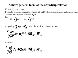
1. A more general form of the Sverdrup relation Ekman layer at bottom Spatially changing sea surface height  and bottom topography zB and pressure pB. Assume atmospheric pressure p≈0. Let , Integrating over the vertical column, we have Similarly

2. Define Ep is the work done to pile up the water above the bottom is the total potential energy of sea water with S=35, T=0oC function of bottom topography only is the potential energy anomaly

3. It can be shown that Therefore, the balance of forces can be written as

4. Define Baroclinic geostrophic transport Barotropic geostrophic transport Ekman transport in the surface layer Ekman transport in the bottom layer Therefore, we have

5. Following Sverdrup’s approach, we take Surface stress curl Bottom stress curl Bottom topography effect Vanish if the bottom is flat Or flow follows topographic contour Net baroclinic geostrophic transport is zero

6. Vorticity Equation In physical oceanography, we deal mostly with the vertical component of vorticity , which is notated as From horizontal momentum equation, (1) (2) Taking , we have

7. For a rotating solid object, the vorticity is two times of its angular velocity

9. Considering the case of constant . For a shallow layer of water (depth H<<L), u and v are not function of z because the horizontal pressure gradient is not a function of z. (In general, the vortex tilting term, is usually small. Then we have the simplified vorticity equation Since the vorticity equation can be written as (ignoring friction) ζ+f is the absolute vorticity

10. Using the Continuity Equation For a layer of thickness H, consider a material column We get or Potential Vorticity Equation

12. Alternative derivation of Sverdrup Relation Construct vorticity equation from geostrophic balance (1)  (2) Integrating over the whole ocean depth, we have is the entrainment rate from the Ekman layer where at 45oN The Sverdrup transport is the total of geostrophic and Ekman transport. The indirectly driven Vg may be much larger than VE.

13. In the ocean’s interior, for large-scale movement, we have the differential form of the Sverdrup relation i.e., ζ<<f

14. Niiler’s (1987) explanation Let us postulate there exists a deep level where horizontal and vertical motion of the water is much reduced from what it is just below the mixed layer (Figure 12.6)... Also let us assume that vorticity is conserved there (or mixing is small) and the flow is so slow that accelerations over the Earth's surface are much smaller than Coriolis accelerations. In such a situation a column of water of depth H will conserve its spin per unit volume, f /H (relative to the sun, parallel to the Earth's axis of rotation). A vortex column which is compressed from the top by wind-forced sinking (H decreases) and whose bottom is in relatively quiescent water would tend to shorten and slow its spin. Thus because of the curved ocean surface it has to move southward (or extend its column) to regain its spin. Therefore, there should be a massive flow of water at some depth below the surface to the south in areas where the surface layers produce a sinking motion and to the north where rising motion is produced. This phenomenon was first modeled correctly by Sverdrup (1947) (after he wrote "Oceans") and gives a dynamically plausible explanation of how wind produces deeper circulation in the ocean.

15. Ekman pumping that produces a downward velocity at the base of the Ekman layer forces the fluid in the interior of the ocean to move southward. From Niiler (1987).

16. Winds at the sea surface drive Ekman transports to the right of the wind in this northern hemisphere example (bold arrows in shaded Ekman layer). The converging Ekman transports driven by the trades and westerlies drives a downward geostrophic flow just below the Ekman layer (bold vertical arrows), leading to downward bowing constant density surfaces ri. Geostrophic currents associated with the warm water are shown by bold arrows. After Tolmazin (1985).