Dynamic Set ADT Binary Trees

1. Dynamic Set ADTBinary Trees Gerda Kamberova Department of Computer Science Hofstra University G.Kamberova, Algorithms

2. Overview • Dynamic set ADT • Some implementations an their complexities • Graphs • Trees • Binary trees (BT) • Binary search trees (BST) • Implementation of Dynamic Set ADT with BST • Complexity of the operations G.Kamberova, Algorithms

3. Dynamic Set ADT • Full set of operations: Min, Max, Predecessor, Successor, Insert, Delete, Search • Implementation • Linked lists: worst-case for search, O(n) • Sorted array: worst-case for insert or delete, O(n) • BST : all operations are O(h) in worst-case, where h is the height of the tree. In worst-case h = n-1. • The height of a randomly built BST with n nodes is O(lg n) Can’t guarantee that a tree is built at random. • Variations of BT that keep the trees balanced achieve O(lg n). Those include AVL trees, Red-black trees, B-trees. B-trees are for maintaining a database on a random access storage G.Kamberova, Algorithms

4. Graphs • Undirected graphG=(V,E) consists of two finite sets • Walk: an alternating sequence of vertices and edges, starting and ending in a vertex, s.t. each edge is incident on the two vertices immediately preceding and following it. • Closed walk: begins and ends at the same vertex • A path: a walk in which no vertex is repeated; the length of the path is the number edges in it • If there is a path from u to v, v is reachable from u • Cycle: closed path • Acyclic graph: without cycles • Connected graph: at least one path exists between every pair vertices G.Kamberova, Algorithms

5. Trees • Tree: connected acyclic graph • Trees are one of the most important data structures • Used to impose hierarchical structure on a problem or collection of data • Rooted tree: one vertex, root, is distinguished from the rest. We will work with rooted trees. • Children of the root: vertices connected to the root with an edge ; the root is a parent of its children. This definition is extended to the children of the root, etc. • The root does not have a parent • Siblings: vertices with the same parent • Leaf (external node): a node with no children • Internal node: vertex other than leaf • Vertex v is a descendent of u, if v is a child of u, or a child of one of the children of u, etc. Then u is an ancestor of v. • All descendents of a vertex form a subtree • Height of a vertex v: the length of the longest path from v to a leaf. Height of the tree is the height of the root. • Depth (level) of a vertex v: the length of the path from the root to v • Ordered tree: siblings are linearly ordered (first, second, etc) G.Kamberova, Algorithms

6. Binary Trees (BT) • BT: an ordered tree in which each vertex has 0, 1 or 2 children • If a vertex has 2 children, the first childe is the “left”, the second is the “right” • If a vertex has one child, it can be positioned either as left or right • If we define an empty tree as a tree with no nodes, a binary tree T, is often defined recursively: T is a BT if • T is empty • T has a left and right subtrees that are BTs • For a node u, parent(u), left(u) and right(u) denote the partme, left and right child of u • Full BT: every vertex has 2 children or is a leaf • Perfect BT: all leaves have the same depth • Complete BT: a BT that is “almost perfect”; what may differentiate it from a perfect tree that is may miss only most right leaves. • K-ary trees: extends the BT concepts to a tree where each node has 0,1,2,3,…, or k children. (BT is 2-ary tree). G.Kamberova, Algorithms

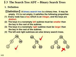
7. BST • BST: a BT in which the keys of the nodes are filled in such a way that satisfy the binary search tree property (BSTP): • for any non-leaf node u, • key(left(u)) < key(u), if left(u) exists • key(u) < key(right(u)), if rightI(u) exists. • Note: • All keys in the left subtree of u are less than key(u) • All keys in the right subtree of u are larger than key(u) • Key values on the same level are sorted in increasing order • For fixed n, max height, n-1, is obtained when the n-node tree is degenerate, and min, \log n, when the tree is complete. m q h c k x a j l G.Kamberova, Algorithms

8. Traversals • visit u means visit the node u and execute specified operations at the node. • Preorder traversal: • Visit the root • Traverse in preorder the left subtree • Traverse in preorder the right subtree • Inorder traversal: • Traverse in inorder the left subtree • Visit the root • Traverse in inorder the righjt subtree • Postorder traversal: • Traverse in postorder the left subtree • Traverse in postorder the right subtree • Visit the root. G.Kamberova, Algorithms

9. BST example traversals • Preorder m, h, c, a, k, j, l, q, x • Inorder a, c, h, j, k, l, m, q, x • Postorder a, c, j, l, k, h, x, q, m m q h c k x a j l G.Kamberova, Algorithms

10. Traversals • Implementation: easy recursively • v is the root iff parent(v)=NULL • v is a leaf iff left(v)=right(v) = NULL • Pseudo code for inorder traversal: inorder(v) // inorder traversal of the BST rooted in v if v is not NULL // if the tree is not empty inorder(left(v)) visit v inorder( right(v) ) • Theorem: Given a BST, T, inorder visits the nodes in sorted order of the keys. Proof: by induction on h G.Kamberova, Algorithms

11. Search • Search a BST for a key k; return the node with key k if found, NULL otherwise. Search(v, k) //search tree rooted in v for key k if v == NULL or k == key(v) return v if k < key(v) Search(left(v), k) else Search(right(v),k) • The vertices encountered during any search are along a path from the root towards a leaf. • Time complexity: in worst case we'll traverse the longest path. thus the Search is O(h). G.Kamberova, Algorithms

12. Search • Iterative implementation Search(v, k) //search tree rooted in v for key k while (v is not NULL and key(v) not equal to k) if key < key(v) v = left(v) else v = right(v) return v G.Kamberova, Algorithms

13. Trace BST search v • search(v,k) returns right(left(v)) • search(v, r) returns right(left(v)) which is null, thus not found m q h null c k x a j l G.Kamberova, Algorithms

14. Min/Max node in BST • Min the node with min key. It is the left-most node (not necessary a leaf) , going down-left from the root : ex “c” • Max is the node with the max key. It the right-most node (not necessary a leaf) going down-right from the root: ex “y” • Implementation maximum(v) while v is not NULL p = v //storeparent v = right(v) return p • Time complexity: O(h). m q h x c k y e j l G.Kamberova, Algorithms

15. Predecessor node of a node in BST Ex: predecessor(v) is w • Predecessor of v: the node with key immediately preceding the key of v,( if exists, otherwise NULL • The ordering is with respect to the sorted keys (the inorder ordering). • Let v be a node s.t. that is has not NULL predecessor, then: • If v has a left subtree, the predecessor of v is the max in left(v). Ex: w • v does not have a left subtree, then the predecessor of v is the most recent ancestor of v which contains v in a right subtree, i.e., the lowest ancestor of v whose right child is also an ancestor of v. (v an ancestor of itself.) m q v h x e k y w g j l u predecessor(u) is v G.Kamberova, Algorithms

16. Predecessor • preddecessor(r, v) finds the predecessor of v in the tree rooted in r. • If it exists, it is either • the max in the left subtree of v, if it left(v) exists, • or it is the lowest ancestor, p, of v whose right child is also an ancestor of v. In this case, from v go up the direct path to the root untill you hit p. • Pseudocode predecessor(r, v) if left(v) is not NULL return maximum(left(v)) p = Parent(v); while (p is not NULL and v == left(p)) v = p p = Parent(p) return p • Time complexity for predecessor and sucessor: O(h) p p p v G.Kamberova, Algorithms

17. Successor node of a node in BST Ex: successor(w) is v • Sucessor of v: the node with key immediately following the key of v,( if exists, otherwise NULL) • The ordering is with respect to the sorted keys (the inorder ordering). • Let v be a node s.t. that is has not NULL successor, then: • If v has a right subtree, the sucessro of v is the min in right(v). • If v does not have a right subtree, then the successor of v is the most recent ancestor of v which contains v in a left subtree, i.e., the lowest ancestor of v whose left child is also an ancestor of v. (v an ancestor of itself.) m q v h h x e k y w g j l u successor(v) is u G.Kamberova, Algorithms

18. Insert a node in BST • To insert a new record : • Create the record to hold the key and the data, and get pointer to it • Find the place in BST where the new object has to be attached • do search for the key to find the place • Attach the new object, making a new leaf as left or right child depending on the key value. • New items are inserted only as leaves. • Ex: insert d, i, o m q h c k x a j l G.Kamberova, Algorithms

19. Insert a node in BST • To insert a new record : • Create the record to hold the key and the data, and get pointer to it • Find the place in BST where the new object has to be attached • do search for the key to find the place • Attach the new object, making a new leaf as left or right child depending on the key value. • New items are inserted only as leaves. • Ex: insert d, i, o m q h c k o x a d j l i G.Kamberova, Algorithms

20. Insert • Example: • build BST tree by successfully inserting in an empty tree 15, 6, 3, 18, 4, 7, 20, 13, 2, 9, 17 • Trace the search on 9, 3, 19 • Find predecessor of node with key 4, 17, 2 • Find successor of node with key 20, 6, 4 G.Kamberova, Algorithms

21. Insert Implementation • Assume that new object has been created, and that u is a pointer to it insert(v, u) { //insert node u in the BST rooted in v // returns the root if v == NULL return v//make v the root // search for place for the new node, as long as not encountered while (v != NULL and key(v)!= key(u)) p = v if key(u) < key(v) v = left(v) else v = right(v) if key(u)<key(p) left(p)=u// insert left else right(p)=u // insert right return v } • Time complexity: clearly $O(h)$ G.Kamberova, Algorithms

22. Delete u • Search for the k • If k is not found do nothing. • If k is found, let u denote the vertex with key k. • Remove the node with key k. There are three cases: • deleting a leaf; • deleting a vertex with one child • deleting a vertex with 2 children • Case 0: u is a leaf, trivial. • Case 1: u has one child; simple, attach the child to parent(u) p • Case 2: u has 2 children • Copy u’s inorder predecessor content over u’s content • Delete the node of the predecessor. • Note that since u has two children, the predecessor m is max in the left subtree, and m has less than 2 children, so deleting the node of the predecessor brings us to one of the two previous cases p m G.Kamberova, Algorithms

23. Example • First by successfully inserting in an empty tree 15, 6, 3, 18, 4, 7, 20, 2, 13, 9, 17 • Next delete: 2, 3, 13, 18 G.Kamberova, Algorithms

24. Example • Build by successfully inserting in an empty tree 15, 6, 3, 18, 4, 7, 20, 2, 13, 9, 17 • Delete 2,3, 13, 18 • Complexity: O(h) 17 15 18 6 4 20 17 7 3 9 4 13 2 9 G.Kamberova, Algorithms

25. Delete Implementation • Assume that node u that contains the key to be deleted has been found, u is not NULL Delete(v, u) //delete u from the subtree v if left(u) == NULL and right(u) == NULL // case 0 if parent(u)==NULL v = NULL // empty tree p = parent(u) if u == left(p) then left child of p is NULL else right child of p is NULL return if left(u)==NULL or right(u)==NULL // case 1 if parent(u)==NULL v=the child of u else p = parent(u) if u == left(p) left child of p = the child of u else right child of p = child of u return q = Maximum(left(u)) // case 2 copy key and data from q to u Delete(v,q) return G.Kamberova, Algorithms

26. Preview of coming attractions • Build a BST from an empty tree by inserting (A,Z,B,Y,C,X,D) in this order • Another approach: chose the keys to be inserted from the sequence given at random • For a randomly constructed BST, BST with random insertions, on average search takes O(lg n) • And another approach: restrict somehow the height of the tree to O(log n), all operations will be O(log n) in worst case. • Obviously insert and delete will have overhead G.Kamberova, Algorithms