Download
1 / 33
330 likes | 488 Views
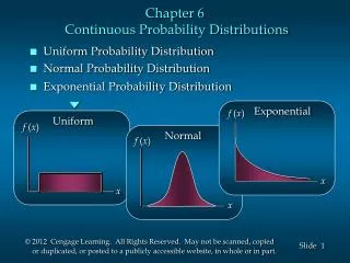
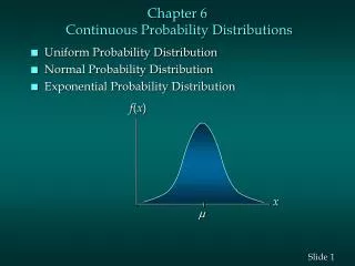
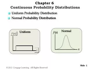
Chapter 6 Continuous Probability Distributions. Figure 6.1 A Discrete Probability Distribution. Probability is represented by the height of the bar. P( x ). 1 2 3 4 5 6 7 x. Holes or breaks between values. f ( x ).

E N D
Figure 6.1 A Discrete Probability Distribution Probability is represented by the height of the bar. P(x) 1 2 3 4 5 6 7 x Holes or breaks between values
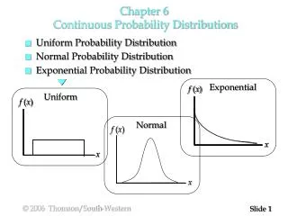
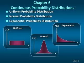
f(x) Probability is represented by area under the curve. x No holes or breaks along the x axis Figure 6.2 A Continuous Probability Distribution
f(x) 1/20 62 72 82 x (commute time in minutes) Figure 6.3 Maria’s Commute Time Distribution
f(x) 1/20 62 64 67 82 x (commute time in minutes) Figure 6.4 Computing P(64 <x< 67) Probability = Area = Width x Height= 3 x 1/20 = .15 or 15%
Total Area = 20 x 1/20 = 1.0 1/20 62 82 20 Figure 6.5 Total Area = 1.0 1/20
Uniform Probability Density Function (6.1) 1/(b-a) for a<x<b f(x) = 0 everywhere else
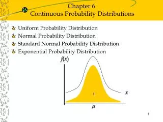
m Figure 6.7 The Bell-Shaped Normal Distribution Mean is m Standard Deviation is s x
Normal Distribution Properties • Approximately 68.3% of the values in a normal distribution will be within one standard deviation of the distribution mean, m. • Approximately 95.5% of the values in a normal distribution will be within two standard deviations of the distribution mean, m. • Approximately 99.7% of the values (nearly all of them) in a normal distribution will be found within three standard deviations of the distribution mean, m.
.683 m-1s m m+1s Figure 6.8 Normal Area for m+ 1s
.955 Figure 6.9 Normal Area for m+ 2s m-2s m m+2s
.997 m-3s m m+3s Figure 6.10 Normal Area for m+ 3s
Figure 6.11 Area in a Standard Normal Distribution for a z of +1.2 .3849 0 1.2 z
m =50 s = 4 .3944 50 55 x (diameter) 0 1.25 z Figure 6.12 P(50 <x< 55)
Figure 6.13 P(x> 58) m =50 s = 4 .0228 .4772 50 58 x(diameter) 0 2.0 z
.2734 .4332 m = 50 s = 4 47 50 56 x(diameter) -.75 0 1.5 z Figure 6.14 P(47 < x < 56)
m = 50 s = 4 .3413 .4772 50 54 58 x (diameter) 0 1.0 2.0 z Figure 6.15 P(54 < x < 58)
Figure 6.16 Finding the z score for an Area of .25 .2500 0 ? z
Exponential Probability (6.7) Density Function f(x) =
Figure 6.17 Exponential Probability Density Function f(x) f(x) =l/elx x
Calculating Area for the (6.8) Exponential Distribution P(x >a) =
f(x) P(x>a) = 1/ela x a Figure 6.18 Calculating Areas for the Exponential Distribution
f(x) P(1.0 <x< 1.5) x 1.0 1.5 Figure 6.19 Finding P(1.0 <x< 1.5)
f(x) P(x> 1.0) = .1354 P(x> 1.5) = .0498 x 1.0 1.5 Figure 6.20 Finding P(1.0 <x< 1.5)
Expected Value for the (6.9) Exponential Distribution E(x) =
Standard Deviation for the (6.11)Exponential Distribution s = =