Download
1 / 34
340 likes | 474 Views
Numerical Libraries for Petascale Computing. Brett Bode William Gropp. Why Use Libraries?. There are many reasons to use libraries: Faster - Code “tricks” Faster – Better Algorithms Correct More productive programming Stuff you don’t want to do

E N D
Numerical Libraries for Petascale Computing Brett Bode William Gropp
Why Use Libraries? • There are many reasons to use libraries: • Faster - Code “tricks” • Faster – Better Algorithms • Correct • More productive programming • Stuff you don’t want to do • There are some reasons not to use libraries • I’ll mention some during the presentation
Faster (Better Code) • Achieving best performance can require creating very processor- and system-specific code • Example: Dense matrix-matrix multiply (DGEMM) • Simple to express: In Fortran, do i=1, n do j=1,n c(i,j) = 0 do k=1,n c(i,j) = c(i,j) + a(i,k) * b(k,j)
Performance Estimate • How fast should this run? • Standard complexity analysis in numerical analysis counts floating point operations • Our matrix-matrix multiply algorithm has 2n3 floating point operations • 3 nested loops, each with n iterations • 1 multiply, 1 add in each inner iteration • For n=100, 2x10⁶ operations, or about 1 msec on a 2GHz processor :) • For n=1000, 2x10⁹ operations, or about 1 sec
The Reality • N=100 • 1818 MF (1.1ms) • N=1000 • 335 MF (6s) • What this tells us: • Obvious expression of algorithms are not transformed into leading performance.
Large gap between natural code and specialized code Hand-tuned Compiler From Atlas Performance Gap in Compiled Code Enormous effort required to get good performance
Sometime Slower • Using a library routine is not always the best choice: • Library routines add overhead • Fewer routines (simpler for user) adds more overhead in determining exact operation • Apply the usual rules: • Instrument your code • Know what performance you need/expect • Only worry about code that takes a significant fraction of the total run time
Faster (Better Code) • Example: Aggregation of operations • Consider • Do i=1,n y(i) = exp(x(i))enddo • Can this be speeded up? • Yes! • Easy – Application requires less accuracy • Harder – Compute multiple exponentials at one time • Overlaps evaluation; share table lookups • Call vexp(y,x,n) • One example: IBM’s libmassv (http://www-01.ibm.com/software/awdtools/mass/)
Faster (Better Algorithms) • Modern algorithms can provide significantly greater performance • Example: Solving systems of linear equations • For most of the history of computing, as much of an improvement in performance in solving systems of linear equations arising from PDEs came from better algorithms as from faster hardware
relative speedup year Algorithms and Moore’s Law This advance took place over a span of about 36 years, or 24 doubling times for Moore’s Law 22416 million the same as the factor from algorithms alone! Thanks to David Keyes for this chart
Example: Multigrid • Multigrid can be a very effective algorithm for certain classes of problems • Efficient implementations must address • Algorithmic choices (e.g., smoother) • Implementation for memory locality • Use as a preconditioner within a Krylov method • And that’s just on a single processor • Parallel versions add questions about efficient coarse grid solves, data exchange, etc. • Libraries such as hypre (https://computation.llnl.gov/casc/linear_solvers/sls_hypre.html) contain efficient implementations for parallel systems
Correct • Some operations are subtle and require care to get them right • Example: (pseudo) random number generation in parallel • Using a local random generator such as srand produces correlated values – not random at all • Simply using different seeds for each thread/process in a parallel program isn’t enough (unless the seeds are picked very carefully) • SPRNG – Scalable Parallel Random Number Generator • Provides good pseudo-random number generators, suitable for use in a parallel program • http://sprng.cs.fsu.edu/
Greater Productivity • Parallel programming is widely viewed as difficult • Much effort to develop programming languages that make parallel programming “easy” • But what is really needed is a way to provide the data structures, algorithms, and methods needed by the computational scientist • A general purpose language is not the best way to do this (though it may be a good way to implement it) • An alternative is through carefully designed libraries…
What Advantage Does This Approach Give You? • Example: A Poisson Solver in PETSc • The following 7 slides show a complete 2-d Poisson solver in PETSc. Features of this solver: • Fully parallel • 2-d decomposition of the 2-d mesh • Linear system described as a sparse matrix; user can select many different sparse data structures • Linear system solved with any user-selected Krylov iterative method and preconditioner provided by PETSc, including GMRES with ILU, BiCGstab with Additive Schwarz, etc. • Complete performance analysis built-in • Only 7 slides of code!
PETSC “objects” hide details of distributed data structures and function parameters Solve a Poisson Problem with Preconditioned GMRES /* -*- Mode: C; c-basic-offset:4 ; -*- */ #include <math.h> #include "petscsles.h" #include "petscda.h" extern Mat FormLaplacianDA2d( DA, int ); extern Vec FormVecFromFunctionDA2d( DA, int, double (*)(double,double) ); /* This function is used to define the right-hand side of the Poisson equation to be solved */ double func( double x, double y ) { return sin(x*M_PI)*sin(y*M_PI); } int main( int argc, char *argv[] ) { SLES sles; Mat A; Vec b, x; DA grid; int its, n, px, py, worldSize; PetscInitialize( &argc, &argv, 0, 0 );
PETSc provides routines to access parameters and defaults PETSc provides routines to create, allocate, and manage distributed data structures /* Get the mesh size. Use 10 by default */ n = 10; PetscOptionsGetInt( PETSC_NULL, "-n", &n, 0 ); /* Get the process decomposition. Default it the same as without DAs */ px = 1; PetscOptionsGetInt( PETSC_NULL, "-px", &px, 0 ); MPI_Comm_size( PETSC_COMM_WORLD, &worldSize ); py = worldSize / px; /* Create a distributed array */ DACreate2d( PETSC_COMM_WORLD, DA_NONPERIODIC, DA_STENCIL_STAR, n, n, px, py, 1, 1, 0, 0, &grid ); /* Form the matrix and the vector corresponding to the DA */ A = FormLaplacianDA2d( grid, n ); b = FormVecFromFunctionDA2d( grid, n, func ); VecDuplicate( b, &x );
PETSc provides routines that solve systems of sparse linear (and nonlinear) equations PETSc provides coordinated I/O (behavior is as-if a single process), including the output of the distributed “vec” object SLESCreate( PETSC_COMM_WORLD, &sles ); SLESSetOperators( sles, A, A, DIFFERENT_NONZERO_PATTERN ); SLESSetFromOptions( sles ); SLESSolve( sles, b, x, &its ); PetscPrintf( PETSC_COMM_WORLD, "Solution is:\n" ); VecView( x, PETSC_VIEWER_STDOUT_WORLD ); PetscPrintf( PETSC_COMM_WORLD, "Required %d iterations\n", its ); MatDestroy( A ); VecDestroy( b ); VecDestroy( x ); SLESDestroy( sles ); DADestroy( grid ); PetscFinalize( ); return 0; }
/* -*- Mode: C; c-basic-offset:4 ; -*- */ #include "petsc.h" #include "petscvec.h" #include "petscda.h" /* Form a vector based on a function for a 2-d regular mesh on the unit square */ Vec FormVecFromFunctionDA2d( DA grid, int n, double (*f)( double, double ) ) { Vec V; int is, ie, js, je, in, jn, i, j; double h; double **vval; h = 1.0 / (n + 1); DACreateGlobalVector( grid, &V ); DAVecGetArray( grid, V, (void **)&vval );
Almost the uniprocess code /* Get global coordinates of this patch in the DA grid */ DAGetCorners( grid, &is, &js, 0, &in, &jn, 0 ); ie = is + in - 1; je = js + jn - 1; for (i=is ; i<=ie ; i++) { for (j=js ; j<=je ; j++){ vval[j][i] = (*f)( (i + 1) * h, (j + 1) * h ); } } DAVecRestoreArray( grid, V, (void **)&vval ); return V; }
Creates a parallel distributed matrix using compressed sparse row format Creating a Sparse Matrix, Distributed Across All Processes /* -*- Mode: C; c-basic-offset:4 ; -*- */ #include "petscsles.h" #include "petscda.h" /* Form the matrix for the 5-point finite difference 2d Laplacian on the unit square. n is the number of interior points along a side */ Mat FormLaplacianDA2d( DA grid, int n ) { Mat A; int r, i, j, is, ie, js, je, in, jn, nelm; MatStencil cols[5], row; double h, oneByh2, vals[5]; h = 1.0 / (n + 1); oneByh2 = 1.0 / (h*h); DAGetMatrix( grid, MATMPIAIJ, &A ); /* Get global coordinates of this patch in the DA grid */ DAGetCorners( grid, &is, &js, 0, &in, &jn, 0 ); ie = is + in - 1; je = js + jn - 1;
Just the usual code for setting the elements of the sparse matrix (the complexity comes, as it often does, from the boundary conditions) for (i=is; i<=ie; i++) { for (j=js; j<=je; j++){ row.j = j; row.i = i; nelm = 0; if (j - 1 > 0) { vals[nelm] = oneByh2; cols[nelm].j = j - 1; cols[nelm++].i = i;} if (i - 1 > 0) { vals[nelm] = oneByh2; cols[nelm].j = j; cols[nelm++].i = i - 1;} vals[nelm] = - 4 * oneByh2; cols[nelm].j = j; cols[nelm++].i = i; if (i + 1 < n - 1) { vals[nelm] = oneByh2; cols[nelm].j = j; cols[nelm++].i = i + 1;} if (j + 1 < n - 1) { vals[nelm] = oneByh2; cols[nelm].j = j + 1; cols[nelm++].i = i;} MatSetValuesStencil( A, 1, &row, nelm, cols, vals, INSERT_VALUES ); } } MatAssemblyBegin(A, MAT_FINAL_ASSEMBLY); MatAssemblyEnd(A, MAT_FINAL_ASSEMBLY); return A; }
On Blue Waters IBM will Provide • Engineering Scientific Subroutine Library (ESSL) • Most BLAS levels 1-3, LAPACK, FFT • Sequential or threaded • Analogous to Intel’s MKL, ATLAS, etc • Parallel ESSL • Analogous to ScaLAPACK • MPI plus subset of ESSL
On Blue Waters IBM will Provide • libmass/libmassv • Mathematical Acceleration SubSystem • Sequential/vector/simd versions • Sequential routines are standard math intrinsic functions – Compiler will attempt to inline mass versions when possible. • simd/vector versions are not portable • Compiler will attempt to generate calls to some routines, but manually calling the library functions is recommended.
Productivity Libraries and Frameworks • Several productivity libraries are receiving special attention for Blue Waters • PETSc (www.mcs.anl.gov/petsc) • Cactus (http://www.cactuscode.org/) • There are many others • Let us know if there are libraries that are important to your applications
Stuff You Don’t Want to Do • Such as Parallel I/O • Common for applications to funnel all I/O through one process • Works around bugsin common file systems such as NFS • Ensures that output is in canonical (natural) format expected by other applications
Portable File Formats • Ad-hoc file formats • Difficult to collaborate • Cannot leverage post-processing tools • MPI provides external32 data encoding • High level I/O libraries • netCDF and HDF5 • Better solutions than external32 • Define a “container” for data • Describes contents • May be queried (self-describing) • Standard format for metadata about the file • Wide range of post-processing tools available
Higher Level I/O Libraries • Scientific applications work with structured data and desire more self-describing file formats • netCDF and HDF5 are two popular “higher level” I/O libraries • Abstract away details of file layout • Provide standard, portable file formats • Include metadata describing contents • For parallel machines, these should be built on top of MPI-IO • HDF5 has an MPI-IO option • http://www.hdfgroup.org/HDF5/
Parallel netCDF (PnetCDF) Cluster PnetCDF • (Serial) netCDF • API for accessing multi-dimensional data sets • Portable file format • Popular in both fusion and climate communities • Parallel netCDF • Very similar API to netCDF • Tuned for better performance in today’s computing environments • Retains the file format so netCDF and PnetCDF applications can share files • PnetCDF builds on top of any MPI-IO implementation • http://trac.mcs.anl.gov/projects/parallel-netcdf ROMIO PVFS2 IBM PnetCDF IBM MPI GPFS
I/O in netCDF and PnetCDF P0 P1 P2 P3 • (Serial) netCDF • Parallel read • All processes read the file independently • No possibility of collective optimizations • Sequential write • Parallel writes are carried out by shipping data to a single process • PnetCDF • Parallel read/write to shared netCDF file • Built on top of MPI-IO which utilizes optimal I/O facilities of the parallel file system and MPI-IO implementation • Allows for MPI-IO hints and datatypes for further optimization netCDF Parallel File System P0 P1 P2 P3 Parallel netCDF Parallel File System
Higher Level Parallel I/O Libraries • PRACs have indicated a need for • MPI-IO • HDF-5 • pnetCDF • Others recognize need for parallel I/O • Many use I/O through one process • Reasons of simplicity, avoid errors/performance problems in concurrent access to a common file • These will need to adapt to other I/O approaches as full performance will require parallel I/O
I/O Library Tuning Issues • No really good parallel I/O benchmarks • IOR, b_eff_io have value but also significant limitations • In particular, application I/O patterns don’t match benchmark patterns • Performance inconsistencies • MPI-IO and pnetCDF should have similar performance • MPI-IO and HDF-5 should have similar performance for data • POSIX I/O and comparable MPI-IO patterns should have similar performance • Performance consistency is important (but not sufficient) for scalability • But performance inconsistencies are common in practice
I/O Library Tuning Activities • Currently developing tests to understand performance inconsistencies • Working with IOR as a basis for tests; extending as necessary • MPI-IO/pnetCDT/HDF-5 tests for both per process performance and for scalability • MPI-IO vs. POSIX for per process performance • These are a necessary first step before focusing on scaling • Also developing correctness tests for concurrent updates to a single file • Test should/will fail for NFS (not POSIX semantics) • Test should not fail for GPFS • But anything not tested isn’t known to work
Recommendations • Don’t do it yourself! • Use Frameworks and Libraries where possible • Exploit principles used in those libraries if you need to write your own • Upgrade existing programs • Much can be done by update/replacing core parts of the application • Embrace multicore – Libraries can be a part of this solution • “MPI everywhere” not a solution • Start over (at least for parts) • Real Petascale may require new algorithms and even mathematical models
Summary • There are many reasons to use libraries: • Faster • Correct • Real parallel I/O • More productive programming • The best reason: they let you focus on getting your science done • There are many libraries available • Only a few mentioned in this talk • Many other good ones available – ask!