Download
1 / 12
120 likes | 124 Views
In this work performance comparison of Time frequency algorithms is presented for removal of Additive White Gaussian Noise. For better time frequency resolution properties and better adaptability of STFT, it is used in this work. Most of the audio sound signals are too large to be processed entirely for Mozart signal of 10 second sampled at 11 KHz will contain 11,000 samples. Processing such a large block of data demands rigorous requirements of hardware and software, also the execution time is very long, hence less speed. Hence data is segmented into blocks and each block of data is then processed individually. The important task is to choose the block length. The signal is segmented into blocks, of optimal length and then, denoising is performed in STFT domain by thresholding the STFT coefficients. When each block is denoised by taking optimal window size or block size, it is further concluded that STFT based algorithm proposed here is superior in terms of quality of the denoised signal and the execution time. It is observed that adaptive block hard type thresholding with STFT gives the best SNR for sound signal. It is further concluded that proposed algorithm performs better than other algorithms in respect of SNR and time of execution. Apoorva Athaley | Papiya Dutta "Audio Signal Denoising Algorithm by Adaptive Block Thresholding using STFT" Published in International Journal of Trend in Scientific Research and Development (ijtsrd), ISSN: 2456-6470, Volume-1 | Issue-6 , October 2017, URL: https://www.ijtsrd.com/papers/ijtsrd2512.pdf Paper URL: http://www.ijtsrd.com/engineering/electronics-and-communication-engineering/2512/audio-signal-denoising-algorithm-by-adaptive-block-thresholding-using-stft/apoorva-athaley<br>

E N D
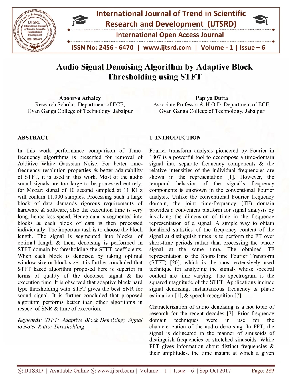
International Research Research and Development (IJTSRD) International Open Access Journal Audio Signal Denoising Algorithm by Adaptive Block Thresholding using STFT International Journal of Trend in Scientific Scientific (IJTSRD) International Open Access Journal ISSN No: 2456 ISSN No: 2456 - 6470 | www.ijtsrd.com | Volume rd.com | Volume - 1 | Issue – 6 Audio Signal Denoising Algorithm Thresholding y Adaptive Block Apoorva Athaley Papiya Dutta Papiya Dutta Research Scholar, Department of ECE, Gyan Ganga College of Technology, Jabalpur Gyan Ganga College of Technology, Jabalpur of ECE, Associate Professor & H.O.D,.Dep Gyan Ganga College of T Gyan Ganga College of Technology, Jabalpur ssociate Professor & H.O.D,.Department of ECE, ABSTRACT In this work performance comparison of Time frequency algorithms is presented for removal of Additive White Gaussian Noise. For better time frequency resolution properties & better adaptability of STFT, it is used in this work. Most of the audio sound signals are too large to be processed entirely; for Mozart signal of 10 second sampled at 11 KHz will contain 11,000 samples. Processing such a large block of data demands rigorous requirements of hardware & software, also the execution time is very long, hence less speed. Hence data is segmented into blocks & each block of data is then processed individually. The important task is to choose the block length. The signal is segmented into blocks, of optimal length & then, denoising is performed in STFT domain by thresholding the STFT coefficients. When each block is denoised by taking optimal window size or block size, it is further concluded that STFT based algorithm proposed here is superior in terms of quality of the denoised signal & the execution time. It is observed that adaptive block hard type thresholding with STFT gives the best SNR for sound signal. It is further concluded that proposed algorithm performs better than other algorithms in respect of SNR & time of execution. 1. INTRODUCTION Fourier transform analysis pioneered by Fourier in 1807 is a powerful tool to decompose a time signal into separate frequency components & the relative intensities of the individual frequencies are shown in the representation [1]. However, the temporal behavior of the signal’s frequency components is unknown in the conventional Fourier analysis. Unlike the conventional Fourier frequency domain, the joint time-frequency (TF) domain provides a convenient platform for signal analysis by involving the dimension of time in the frequency representation of a signal. A simple way to obtain localized statistics of the frequency content of the signal at distinguish times is to perform the FT over short-time periods rather than processing the whole signal at the same time. The o representation is the Short-Time Fourier Transform (STFT) [20], which is the most extensively used technique for analyzing the signals whose spectral content are time varying. The spectrogram is the squared magnitude of the STFT. Applications in signal denoising, instantaneous frequency & phase estimation [1], & speech recognition [7]. estimation [1], & speech recognition [7]. In this work performance comparison of Time- frequency algorithms is presented for removal of Additive White Gaussian Noise. For better time- frequency resolution properties & better adaptability Fourier transform analysis pioneered by Fourier in 1807 is a powerful tool to decompose a time-domain signal into separate frequency components & the elative intensities of the individual frequencies are shown in the representation [1]. However, the temporal behavior of the signal’s frequency components is unknown in the conventional Fourier analysis. Unlike the conventional Fourier frequency work. Most of the audio sound signals are too large to be processed entirely; for Mozart signal of 10 second sampled at 11 KHz will contain 11,000 samples. Processing such a large block of data demands rigorous requirements of frequency (TF) domain execution time is very provides a convenient platform for signal analysis by involving the dimension of time in the frequency representation of a signal. A simple way to obtain of the frequency content of the signal at distinguish times is to perform the FT over time periods rather than processing the whole signal at the same time. The obtained TF long, hence less speed. Hence data is segmented into blocks & each block of data is then processed individually. The important task is to choose the block The signal is segmented into blocks, of ing is performed in STFT domain by thresholding the STFT coefficients. When each block is denoised by taking optimal window size or block size, it is further concluded that STFT based algorithm proposed here is superior in Time Fourier Transform (STFT) [20], which is the most extensively used technique for analyzing the signals whose spectral content are time varying. The spectrogram is the squared magnitude of the STFT. Applications include signal denoising, instantaneous frequency & phase signal & the execution time. It is observed that adaptive block hard type thresholding with STFT gives the best SNR for sound signal. It is further concluded that proposed algorithm performs better than other algorithms in Characterization of audio denoising is a hot topic of research for the recent decades [7]. Prior frequency domain techniques were ion of the audio denoising. In FFT, the signal is delineated in the manner of sinusoids of distinguish frequencies or stretched sinusoids. While FFT gives information about distinct frequencies & Characterization of audio denoising is a hot topic of research for the recent decades [7]. Prior frequency domain techniques were characterization of the audio denoising. In FFT, the signal is delineated in the manner of sinusoids of distinguish frequencies or stretched sinusoids. While FFT gives information about distinct frequencies & their amplitudes, the time instant at which a given their amplitudes, the time instant at which a given Keywords: STFT; Adaptive Block Denoising; Signal to Noise Ratio; Thresholding STFT; Adaptive Block Denoising; Signal in in use use for for the the @ IJTSRD | Available Online @ www.ijtsrd.com @ IJTSRD | Available Online @ www.ijtsrd.com | Volume – 1 | Issue – 6 | Sep-Oct 2017 Oct 2017 Page: 289
International Journal of Trend in Scientific Research and Development (IJTSRD) ISSN: 2456-6470 frequency component occurs cannot be determined. To prevail over this problem, Short-Time Fourier Transform (STFT) technique However, in STFT designing optimal window size for a given application is not so simple [10]. For small window size, sinusoids are not fully resolved & some energy fluctuations are observed; for larger window size all sinusoids are resolved but time localization of sinusoids is not accurate. The noise free signal obtained after “wavelet transformation techniques is not fully free from noise, means some residues of noise are left or any other kinds of noise is generated by the transformation which affects the output signal. Several techniques were introduced to remove the residual noise from the signal; however, the efficiency remains an issue [13]. In [10], a signal denoising technique which is based in transformation domain on block matching technique was proposed. The improvement of the block matching is obtained by grouping same type of segments of the audio into a set of multidimensional arrays. Due to the similarities in these segments or blocks, the transformation can achieve a better reproduction of the original signal. was developed. Figure 1: Comparison of STFT with other transforms Signal Denoising In signal processing removal of noise from signal is very tedious job. An undesired signal when overlapped to a clean signal makes it distorted. How one can extract the original signal & remove the overlapped signal without deterioration of original clean signal. Many algorithms were developed for efficient removal of noise in various applications. The technique used to denoise the signal gets more advanced when the regularity of noise is reduced. When signals pass communicating medium, the noise is added naturally which results in signal contamination. It is tuff to remove this unwanted signal. Hence, the major task in signal processing is to denoise the audio signal with minimum quality degradation of the original signal. The major cause for pollution in audio sound signals is the humming distortion from audio equipments or buzzing & environmental noise [15]. Hence, attenuation of noise while reconstructing the underlying signals is the primary objective of audio denoising. A general denoising technique based on STFT coefficients contraction [15] basically consists of three steps; 1.Apply STFT to noisy signal as; ?.? = ?.? + ?.? from equipments & Where; y, s, z & W are the resultant noisy audio, clean audio signal, noise signal & the matrix associated to the STFT respectively. 2.Thresholding is done for the obtained transformed coefficients. 3.The final denoised version of the signal is reconstructed by ISTFT to the thresholded STFT coefficients. The continuous Short-Time Fourier Transform (STFT) analysis of a signal ?(?) can be obtained as [10]: ?????(?,?;ℎ) = ∫ℎ∗(? − ?)?(?)??????? @ IJTSRD | Available Online @ www.ijtsrd.com | Volume – 1 | Issue – 6 | Sep-Oct 2017 Page: 290
International Journal of Trend in Scientific Research and Development (IJTSRD) ISSN: 2456-6470 yield results that’s are competitive with other audio denoising approaches. approach retains a small percentage of the transform signal coefficients in representation, i.e., it produces very sparse denoised results. Notably, the proposed building a denoised [3] Richard E. Turner, Maneesh Sahani, “Time- Frequency Analysis as Probabilistic Inference”, IEEE transaction on signal Number-23, 2014. processing, Volume-62, This paper proposes a new view of time-frequency analysis framed in terms of probabilistic inference. Natural signals are assumed to be formed by the superposition of distinct time-frequency components, with the analytic goal being to infer these components by application of Bayes’ rule. The framework serves to unify various existing models for natural time- series; it relates to both the Wiener and Kalman filters, and with suitable assumptions yields inferential interpretations of the short-time Fourier transform, spectrogram, filter bank, and wavelet representations. Value is gained by placing time- frequency analysis on the same probabilistic basis as is often employed in applications such as denoising, source separation, or recognition. Uncertainty in the time-frequency representation can be propagated correctly to application-specific stages, improving the handing of noise and missing data. Figure 2: Signal Denoising Example 2. LITERATURE REVIEW [1] Ilker Bayram, “Employing phase information for audio denoising”, IEEE International Conference on Acoustic, Speech and Signal Processing (ICASSP), 2014. In this paper, authors propose a scheme that takes into account the phase information of the signals for the audio denoising problem. The scheme requires to minimize a cost function composed of a diagonally weighted quadrature data term and a fused-lasso type penalty. They have formulated the problem as a saddle point search problem and propose an algorithm that numerically finds the solution. Based on the optimality conditions of the problem, we present a guideline on how to select the parameters of the problem. [4] S. S. Joshi and Dr. S. M. Mukane, “Comparative Analysis of Thresholding Techniques using Discrete Wavelet Transform”, International Electronics Communication Engineering, Volume 5, Issue (4) July, 2014. Journal Computer of and This paper about to reduce the noise by Adaptive time-frequency Block Thresholding procedure using discrete wavelet transform to achieve better SNR of the audio signal. Discrete-wavelet transforms based algorithms are used for audio signal denoising. The resulting algorithm is robust to variations of signal structures such as short transients and long harmonics. Analysis is done on noisy speech signal corrupted by white noise at 0dB, 5dB, 10dB and 15dB signal to noise ratio levels. Here, both hard thresholding and soft thresholding are used for denoising. Simulation & results are performed in MATLAB 7.10.0 (R2010a). In this paper they compared results of soft thresholding and hard thresholding [2] Gautam Bhattacharya, Philippe Depalle, “Sparse denoising of audio by greedy time-frequency shrinkage”, IEEE International Conference on Acoustic, Speech and Signal Processing (ICASSP), 2014. This work presents an analysis of MP in the context of audio denoising. By interpreting the algorithm as a simple shrinkage approach, we identify the factors critical to its success, and propose several approaches to improve its performance and robustness. They have presented experimental results on a wide range of audio signals, and show that the method is able to @ IJTSRD | Available Online @ www.ijtsrd.com | Volume – 1 | Issue – 6 | Sep-Oct 2017 Page: 291
International Journal of Trend in Scientific Research and Development (IJTSRD) ISSN: 2456-6470 [5] Kwang Myung Jeon et-al, “An MDCT-Domain Audio Denoising Method with a Block Switching Scheme”, IEEE Transactions Electronics, Vol. 59, No. 4, November 2013. coefficient is greater than λ, then it is assumed that it is significant and contributes to the original signal. Otherwise it is due to the noise and discarded. The soft thresholding function shrinks the coefficients by λ towards zero. Hence this function is also called as block shrinkage function. The soft thresholding function is defined as: on Consumer In this paper, an audio denoising method is proposed for improving the quality of handheld audio recording devices. The proposed method reduces noise differently depending on the block size in the modified discrete cosine transform (MDCT) analysis of an audio coder. Specifically, denoising for a long block is performed by multi-band spectral subtraction (MBSS) with perceptually weighted scale-factor bands, while that for a short block is performed by subband power scaling to maintain coherence of power with the previously-denoised long block. In order to evaluate the performance of the proposed method, it is first embedded into MPEG-2 advanced audio coding (AAC) that is popularly used for audio recording devices. In [13], we see that the soft thresholding gives lesser mean square error for image signals. Due to this reason soft thresholding is preferred over hard thresholding in case of image processing, but in case of audio signals, we could see that hard thresholding results in lesser amount of mean square error. 3.2 Block Selection Most of the musical instrument sound signals are far too long to be processed in their entirety; for example, a 10 second sound signal sampled at 44.1 KHz will contain 441,000 samples. Thus, as with spectral methods of noise reduction, it is necessary to divide the time domain signal in multiple blocks and process each block individually. The block formation of the signal is shown in the Figure 3. The important task is to choose the block length. Berger et al. [14] shows that, blocks which are too shorts fail to pick important time structures of the signal. Conversely, blocks which are too long miss cause the algorithm to miss the important transient details in the musical instrument sound signal. Due to the binary splitting nature of the tree bases in wavelet analysis to decompose the signal, it is better to choose the length of each block with a number of samples to a power of two. 3. STATE OF ART OF AUDIO DENOISING A noise reduction technique developed by donoho, uses the STFT coefficients contraction and its principle consists of three steps; 1) Apply discrete wavelet transform to noisy signal: W.y =W.s + W.z (5) 2) Threshold the obtained STFT coefficients. 3) Reconstruct the desired signal by applying the inverse STFT to the thresholded STFT coefficients. If the audio signal f is corrupted by a noise w which is often modeled as a zero mean Gaussian process independent of f: ?[?] = ?[?] + ?[?], ? = 0,1…………? − 1 3.1 Thresholding The thresholding function which is also known as shrinkage function is categorized as hard thresholding and soft thresholding function. The hard thresholding function retains the wavelet coefficients which are greater than the threshold λ and sets all other to zero. The hard thresholding is defined as: Figure 3: Block Formation of a Signal As discussed previously, the block size chosen must strike a balance between being able to pick up important transient detail in the sound signal, as well as recognizing longer duration, sustained events. Tables 1 shows the PSNR values which are quality The threshold λ is chosen according to the signal energy and the standard deviation σ of the noise. If the @ IJTSRD | Available Online @ www.ijtsrd.com | Volume – 1 | Issue – 6 | Sep-Oct 2017 Page: 292
International Journal of Trend in Scientific Research and Development (IJTSRD) ISSN: 2456-6470 measures, obtained for various block sizes and for different signals. where Th is threshold value, Lj is the length of each block of noisy signal and k is the constant whose value is varying between 0 - 1. For determining the optimum threshold, value of k should be estimated. 3.3. Threshold Selection Donoho and Johnstone derived a general optimal universal threshold for the Gaussian white noise under a mean square error (MSE) criterion described in [12]. However, this threshold is not ideal for musical instrument sound signals due to poor correlation between the MSE and subjective quality and the more realistic presence of correlated noise. Here we use a new time frequency dependent threshold estimation method. In this method first of all the standard deviation of the noise, σ is calculated for each block. For given σ, we calculate the threshold for each block. Noise component removal by thresholding the wavelet coefficients is based on the observation that in musical instrument sound signal, energy is mostly concentrated in small number of wavelet dimensions. The coefficients of these dimensions are relatively very large compared to other dimensions or to any other signal like noise that has its energy spread over a large number of coefficients. Hence by setting smaller coefficients to be zero, we can optimally eliminate noise while information of the signal. In wavelet domain noise is characterized by smaller coefficients, while signal energy is concentrated in larger coefficients. This feature is useful for eliminating noise from signal by choosing the appropriate threshold. Generally the selected threshold is multiplied by the median value of the detail coefficients at some specified level which is called threshold processing. 3.4 Choice of Thresholding Level λ: Given a choice of block size and the residual noise probability level δ that one tolerates, the thresholding level λ .For each block width and length, λ is estimated using “Monte Carlo simulation“ [15]. Table 1 shows the resulting λ with δ = 0.1%. Let us remark that for a block width W > 1, blocks that contain same number of coefficients, B# = LXW , have close λ values [15]. λ value W = 16 W = 8 W = 4 W = 2 W = 1 L = 8 1.5 1.6 1.9 2.3 2.5 L = 4 1.7 1.9 2.4 3.0 3.4 L = 2 1.9 2.5 3.4 3.2 4.8 Table 1. Thresholding level λ for different block size [15] preserving important The partition of macro blocks in to blocks of different sizes is as shown below: At each level of decomposition, the standard deviation of the noisy signal is calculated. The standard deviation is calculated by Equation (8): (8) where cj are high frequency wavelet coefficients at jth level of decomposition, which are used to identify the noise components and σj is Median Absolute Deviation (MAD) at this level. This standard deviation can be further used to set the threshold value based on the noise energy at that level. The modified threshold value [15] can be obtained by the equation (9): Figure 4: Partition of macroblocks into blocks of different sizes The adaptive block thresholding chooses the sizes by minimizing an estimate of the risk. The risk cannot be calculated since is unknown, but it can be estimated with Stein risk estimate. The adaptive block thresholding groups coefficients in blocks whose sizes (9) @ IJTSRD | Available Online @ www.ijtsrd.com | Volume – 1 | Issue – 6 | Sep-Oct 2017 Page: 293
International Journal of Trend in Scientific Research and Development (IJTSRD) ISSN: 2456-6470 are adjusted to minimize the Stein risk estimate and it attenuates coefficients in those blocks [15]. For audio signal denoising, an adaptive block thresholding non- diagonal estimator is described that automatically adjusts all parameters. It relies on the ability to compute an estimate of the risk, with no prior stochastic audio signal model, which makes this approach particularly robust. Thus, an adaptive audio block thresholding algorithm that adapts all parameters to the time-frequency regularity of the audio signal. The adaptation is performed by minimizing a Stein unbiased risk estimator calculated from the data. The resulting algorithm is robust to variations of signal structures such as short transients and long harmonics. The coefficients (soft/hard thresholding}. The adaptive block thresholding chooses the Block sizes by minimizing an estimate of the risk. ??,? = 1,2,…….,? as illustrated in Figure 3. Each macroblock ?? is segmented in blocks ??of same size which means that ?? macroblock??. The Stein over ??is(1 ? ⁄ )∑ ??? ?∈?? . Several such segmentations are possible & we want to choose the one that leads to the smallest risk estimation [15]. The optimal block size & hence ?? is calculated by choosing the block shape that minimizes ∑ ?∈?? are computed, coefficients in each ??are attenuated with ??= 1 − #= ?? is constant over a risk estimation ??? . Once the block sizes ? ????? where λ is calculated with; ????{∈ ??> ???} = ? 4.1 Proposed Algorithm The proposed STFT based block denoising algorithm for reduction of AWGN is explained in the following steps: 1. Take an input sound signal of desired length, which is suitable. 2. Add “White Gaussian Noise” to the original signal accordance with the standard deviation. 3. Divide the resultant noisy signal data into blocks of different length &accordance with the length of the data in time domain; preferably, number of samples, N, 2M where M is an integer. 4. Calculate Mean Square Error of each of these blocks by; ? 4. PROPOSED METHODOLOGY A block thresholding is the method of segmenting the time-frequency plane into disjoint rectangular blocks of width in frequency & length in time. The choice of block size & shape among various possibilities is called as “block size”. The adaptive block thresholding is the technique that choose the size by reducing an estimated risk. The risk ? ??? − ??can’t be computed as it is not known but can be ??? estimated through Stein risk estimator. Best block sizes are computed by minimizing the estimated risk. If the noise is Gaussian white & the frame is an orthogonal basis then the noise coefficients are uncorrelated with same variance & Stein theorem proves that is an unbiased risk estimator of the risk. Hence, if the noise isn’t white in nature & if it is stationary then the variance doesn’t vary in time. If the blocks ?? are sufficiently narrow in frequency then the variance remains unchanged over each block so the risk estimator remains unbiased & a tight frame acts as a union of orthogonal bases. As a consequence, the theorem approximately & the resulting estimator mains nearly unbiased. In the adaptive block thresholding, coefficients are grouped in blocks where size is adjusted to minimize the Stein estimated risk. Firstly decomposition of time-frequency plane into macroblocks is done to regularize the adaptive segmentation in blocks, ??? =1 ??[??(?) − ??(?)]? ??? Where; ? is the length of the signal. 5. Optimal block is the one resulting in minimum mean square error. 6. Compute the “Short Time Fourier Transform (STFT)” of one block of the noisy signal at first level. 7. Estimate the standard deviation of the noise using; ??=?????? ?????? 0.6745 & determine the threshold value using; result applies ?ℎ= ? ∗ ???2????????????? @ IJTSRD | Available Online @ www.ijtsrd.com | Volume – 1 | Issue – 6 | Sep-Oct 2017 Page: 294
International Journal of Trend in Scientific Research and Development (IJTSRD) ISSN: 2456-6470 ? ? Then apply the hard thresholding method for time & level dependent STFT coefficients using; ?ℎ(?) = ??, |?| ≥ ? 0, ??ℎ?????? 8. Take “Inverse Short Time Fourier Transform (ISTFT)” of the noise free coefficients achieved through iterative loop from previous step, which are denoised version using proposed algorithm. 9. Calculate performance parameters used for audio performance indication like MSE, SNR, MAE & CC of the denoised signal. ??? =1 ??|??− ?| =1 ??? ?|??| ? ??? The MAE is the averaging of absolute errors |??| = |??− ?|, where ?? is the forecast & ? is the original value. 4.3 Proposed Algorithm Flow Chart 4.2 Performance Parameters SNR: For comparing measurement of quality of denoising, the “Signal to Noise Ratio (SNR)” is determined between the original signal?? & the denoised signal ??, by our proposed algorithm. The SNR is calculated as; the performance and ? ??? = 10?????????? ???? Figure 4: Proposed STFT based Audio Denoising Algorithm Where; ???? is the maximum value of the signal & is given by, 5. RESULTS AND DISCUSSIONS In this work all the simulations have been done in MATLAB 7.1. Signal Processing toolbox of MATLAB along with other general toolboxes has been used for coding in MATLAB. Standard Mozart.wav is taken as the test audio signal, since it is broadly used in literatures for testing purpose of audio denoising algorithm. First we have taken this audio signal & then AWGN noise with known variance is added, then our proposed Thresholding algorithm by using STFT is applied to it. Simulation gives SNR of the noisy signal is 5 dB & SNR of the denoised signal is 15.47 dB by our proposed method for Mozart sample at 11 KHz & Noisy sample of Mozart at -5dB AWGN with 0.047 noise variance. ????= max (max(??),max(??)) Cross-correlation: It is used in signal processing as a tool to find similarity between two signals. It is also called as a sliding inner-product or sliding dot product. It is generally used in time-series analysis for finding a large signal for smaller &known features. For continuous functions ?&??, the cross-correlation is defined as: ∞ Adaptive block ? ∗ ??≝ ??∗(?)??(? + ?) ??, ?∞ Where ?∗denotes the complex conjugate of ?&? is the lag. Similarly, for discrete functions, the cross- correlation is defined as: ∞ (? ∗ ??)[?] ≝ ? ?∗[?]??[? + ?] ???∞ MAE: The Mean Absolute Error (MAE) is a quantitative parameter which is used find closeness of the predictions. In time series analysis the MAE is a general tool for predicting errors. The formulation of mean absolute error is given by: 5.1 Spectrogram Analysis The STFT’s squared magnitude or spectrogram can be achieved by using kernel equal to an analysis short- time window. The short-time energy-density spectrum can be obtained as the squared magnitude of STFT & is commonly called the spectrogram. When a unit- @ IJTSRD | Available Online @ www.ijtsrd.com | Volume – 1 | Issue – 6 | Sep-Oct 2017 Page: 295
International Journal of Trend in Scientific Research and Development (IJTSRD) ISSN: 2456 International Journal of Trend in Scientific Research and Development (IJTSRD) ISSN: 2456 International Journal of Trend in Scientific Research and Development (IJTSRD) ISSN: 2456-6470 energy window is used then the total energy of the spectrogram equals that of the signal. For audio signal time-frequency representation spectrogram is quite commonly used. energy window is used then the total energy of the spectrogram equals that of the signal. For audio frequency representation spectrogram is 5.1.3 Spectrogram of Denoised Audio (at 5dB) of Denoised Audio (at 5dB) 5.1.1 Spectrogram of Clean Audio Figure 7: Spectrogram of Denoised Audio Figure 7: Spectrogram of Denoised Audio 5.1.4 Spectrogram of Noisy Audio (at 15 dB) 5.1.4 Spectrogram of Noisy Audio (at 15 dB) Figure 5: Spectrogram of Clean Audio gram of Clean Audio Figure 5 shows clean audio has some high frequency, low amplitude components, which will become problematic when noise will be added. Figure 5 shows clean audio has some high frequency, low amplitude components, which will become 5.1.2 Spectrogram of Noisy Audio (at 5dB) 5.1.2 Spectrogram of Noisy Audio (at 5dB) Figure 8: Spectrogram of Noisy Audio Figure 8: Spectrogram of Noisy Audio 5.1.5 Spectrogram of Denoised Audio (at 15 dB) 5.1.5 Spectrogram of Denoised Audio (at 15 dB) Figure 6: Spectrogram of Noisy Audio Figure 6: Spectrogram of Noisy Audio Figure 9: Spectrogram of Denoised Audio Figure 9: Spectrogram of Denoised Audio @ IJTSRD | Available Online @ www.ijtsrd.com @ IJTSRD | Available Online @ www.ijtsrd.com | Volume – 1 | Issue – 6 | Sep-Oct 2017 Oct 2017 Page: 296
International Journal of Trend in Scientific Research and Development (IJTSRD) ISSN: 2456-6470 5.1.6 Spectrogram of Noisy Audio (at 25 dB) 5.2 Amplitude Spectrum Analysis 5.2.1 Amplitude Spectrum of Original vs Noisy Signal Figure 10: Spectrogram of Noisy Audio Figure 10 shows spectrogram of the audio after corrupted with 25 dB AWGN i.e. noise variance σ=0.0047, which also has very dense high frequency & low amplitude components, which are more effected with noise, which will further cause musical noise. It can be seen from figure that noise density is furthermore, as compared to 15 dB. Figure 12: Amplitude Spectrum of Original vs Noisy Signal 5.2.2 Amplitude Spectrum of Noisy vs Denoised Signal 5.1.7 Spectrogram of Denoised Audio (at 25 dB) Figure 13: Amplitude Spectrum of Noisy vs Denoised Signal Figure 11: Spectrogram of Denoised Audio Figure 11 shows the spectrogram of denoised audio with our proposed algorithm, it can be clearly seen that musical noise or high frequency low amplitude components has been eliminated after denoising process. SNR of the denoised signal is 31.18 dB, with 0.000007 MSE, 0.002096 MAE & cross-correlation of 0.999, which are further improved with 15 dB performance. @ IJTSRD | Available Online @ www.ijtsrd.com | Volume – 1 | Issue – 6 | Sep-Oct 2017 Page: 297
International Journal of Trend in Scientific Research and Development (IJTSRD) ISSN: 2456-6470 5.2.3 Amplitude Spectrum of Original vs Denoised Signal Figure 16: MSE Performance after Denoising Figure 14: Amplitude Spectrum of Original vs Denoised Signal 5.3 Simulation Results Summary Table 2: Simulation Results Summary of the Proposed Work In this work simulations have been done for various values of noise variance (σ) from 5 dB to 25 dB & various parameters for noisy & denoised signals are listed in table 2. The noise added to the original signal is AWGN (Additive White Gaussian Noise). The above table is for Mozart.wav audio, as in the literature this signal is most commonly used. From the above table it can be clearly seen that all the parameters like MSE, MAE, SNR, & PSNR & CC are improved for denoised signal as compared to the noisy Figure 17: MAE Performance after Denoising signal. Figure 18: Cross Correlation Performance after Denoising 5.4 Performance Comparison Performance comparison of Block Thresholding (BT), mentioned in the [1] of Mozart audio signal for the Figure 15: SNR Performance after Denoising @ IJTSRD | Available Online @ www.ijtsrd.com | Volume – 1 | Issue – 6 | Sep-Oct 2017 Page: 298
International Journal of Trend in Scientific Research and Development (IJTSRD) ISSN: 2456-6470 various SNR values is depicted below in table 3. It shows improvement in SNR with proposed work with [1] for all values of noise variance. length. The signal is segmented into blocks, of optimal length & then, denoising is performed in STFT domain by thresholding the STFT coefficients. When each block is denoised by taking optimal window size or block size, it is further concluded that STFT based algorithm proposed here is superior in terms of quality of the denoised signal & the execution time. It is observed that adaptive block hard type thresholding with STFT gives the best SNR for sound signal. It is further concluded that proposed algorithm performs better than other algorithms in respect of SNR & time of execution. REFERENCES [1] Ilker Bayram, “Employing phase information for audio denoising”, IEEE International Conference on Acoustic, Speech and Signal Processing (ICASSP), 2014. Table 3: Performance Comparison of Previous Work with Proposed Work [2] Gautam Bhattacharya, Philippe Depalle, “Sparse denoising of audio by greedy time-frequency shrinkage”, IEEE International Conference on Acoustic, Speech and Signal Processing (ICASSP), 2014. [3] Richard E. Turner, Maneesh Sahani, “Time- Frequency Analysis as Probabilistic Inference”, IEEE transaction on signal Number-23, 2014. processing, Volume-62, Figure 19: Performance Comparison of Base Paper Work with Proposed Work [4] S. S. Joshi and Dr. S. M. Mukane, “Comparative Analysis of Thresholding Techniques using Discrete Wavelet Transform”, International Electronics Communication Engineering, Volume 5, Issue (4) July, 2014. From the table 3 & figure 19, the improvement in SNR of our proposed algorithm can be clearly seen compared to the results of base paper [1]. Journal Computer of and [5] Kwang Myung Jeon et-al, “An MDCT-Domain Audio Denoising Method with a Block Switching Scheme”, IEEE Transactions Electronics, Vol. 59, No. 4, November 2013. 6. CONCLUSION In this work performance comparison of Time- frequency algorithms is presented for removal of Additive White Gaussian Noise. For better time- frequency resolution properties & better adaptability of STFT, it is used in this work. Most of the audio sound signals are too large to be processed entirely; for Mozart signal of 10 second sampled at 11 KHz will contain 11,000 samples. Processing such a large block of data demands rigorous requirements of hardware & software, also the execution time is very long, hence less speed. Hence data is segmented into blocks & each block of data is then processed individually. The important task is to choose the block on Consumer [6] “Implementation Thresholding Algorithm in Audio Noise Reduction”, International Journal of Science, Engineering and Technology Research (IJSETR), Volume 2, Issue 7, July 2013. K.P. Obulesu and Time P. Uday Kumar, Block of Frequency [7] Jagadale, B. N., “Audio signal processing using wavelet transform,” Journal of Computer and Mathematical Sciences, Vol. 3, No. 6, pp. 557- 663, 2012. @ IJTSRD | Available Online @ www.ijtsrd.com | Volume – 1 | Issue – 6 | Sep-Oct 2017 Page: 299
International Journal of Trend in Scientific Research and Development (IJTSRD) ISSN: 2456-6470 [8] Jain, S. N., and Rai, C., “Blind source separation and ICA techniques: a review,” International Journal of Engineering Science and Technology, Vol. 4, No. 4, pp. 1490-1503, 2012. [18] Bakirci, U., and Kucuk, U., “The compression of musical instrument signals by wavelet transform,” IEEE Proceedings of International Conference on Signal Processing and Communications Applications, pp. 493-495, 2004. [9] Nehe, N. S., and Holambe, R. S., “DWT and LPC based feature extraction methods for isolated word recognition,” EURASIP Journal of Audio, Speech and Music Processing, Springer, pp. 1-7, 2012. [19] Chevalier, P., Albera, L., Comon, P., and Ferreol, A., “Comparative performance analysis of eight blind source separation methods on radio communication signals,” IEEE International Joint Conference on Neural Networks, 2004. [10] Cohen, R., “Signal denoising using wavelets,” Project Report, Israel Institute of Technology, 2012. [20] Ching, T., and Wang, H. C., “Enhancement of single channel speech based on masking property and wavelet transform,” Speech Communications, Vol. 41, No. 2, pp. 409-427, 2003. [11] Alam, M., Islam, M. I., and Amin, M. R., “Performance comparison of STFT, WT, LMS and RLS adaptive algorithms in denoising of speech signals,” International Journal of Engineering and Technology, Vol. 3, No. 3, pp. 235-238, 2011. [21] Asano, F., Ikeda, S., Ogawa, M., Asoh, H., and Kitawaki, N., “Combined approach of array processing and independent component analysis for blind separation of acoustic Transactions on Speech & Audio Processing, Vol. 11, No. 3, 2003. [12] Chen, D., Maclachlan, S., and Kilmer, M., “Iterative parameter choice and multigrid methods for anisotropic diffusion denoising,” SIAM Journal of Scientific Computing, Vol. 33, No. 5, pp. 2972-2994, 2011. signals,” IEEE [22] Alam, J. F., and Walker, J. S., “Time frequency analysis of musical instruments,” Proceedings in Society of Industrial and Applied Mathematics, Vol. 44, No. 3, pp. 457-476, 2002. [13] Basumallick, N., and Narasimhan, S. V., “A discrete cosine adaptive harmonic wavelet packet and its application to signal compression,” Journal of Signal and Information Processing, Vol. 1, Pp. 63-67, 2010. [23] Antoniadis, A., Bigot, J., and Sapatinas, T., “Wavelet estimators in nonparametric regression: A comparative simulation study,” Journal of Statistical Software, Vol. 6, No. 6, pp. 1-83, 2001. [14] Abid, K., Ouni, K., and Ellouze, N., “A new psychoacoustic model for MPEG1 layer 3 coder using a dynamic gammachirp wavelet,” IEEE Proceedings of International Conference on Signal Processing and Information Technology, pp. 123-128, 2009. [24] Dapena, A., Bugallo, M. F., and Castedo, L., “Separation of convolutive mixtures of temporally- white signals: A novel frequency-domain approach,” Proceedings of International Independent Component Analysis Blind Source Separation, pp. 315-320, 2001. [15] Guoshen Yu, Stéphane Mallat, and Emmanuel Bacry, “Audio Denoising by Time-Frequency Block Thresholding”, IEEE Transactions Processing, Vol. 56, No. 5, 2008. Conference on on Signal [25] Batista, L. V., Melcher, E., and Carvalho, L. C., “Compression of ECG signals by optimized quantization of discrete coefficients,” Journal of Medical Engineering Physics, Vol. 23, No. 2, pp.127-134, 2001. [16] Castells, F., Laguna, P., Srnmo, L., and Bollmann, A., “Principle component analysis in ECG signal processing,” EURASIP Journal of Applied Signal Processing, pp. 1-21, 2007. cosine transform [17] Bahoura, M., and Rouat, J., “Wavelet speech enhancement based on time-scale adaptation,” Speech Communications, Vol. 48, No. 12, pp. 1620-1637, 2006. @ IJTSRD | Available Online @ www.ijtsrd.com | Volume – 1 | Issue – 6 | Sep-Oct 2017 Page: 300