Download
1 / 71
710 likes | 834 Views
From Endogenous Firms to Macro-Volatility with 120 million Agents. Rob Axtell Krasnow Institute for Advanced Study George Mason. Transition in the Social Sciences. Decision theory Rational actors: Utility maximization Profit maximization Representative agents Indirect interactions

E N D
From Endogenous FirmstoMacro-Volatilitywith120 million Agents • Rob Axtell • Krasnow Institute for Advanced Study • George Mason
Transition in the Social Sciences • Decision theory • Rational actors: • Utility maximization • Profit maximization • Representative agents • Indirect interactions • Agent-level equilibrium • Ag data + econometrics • OR and optimization • Top down AI • Game theory • Behavioral economics: • Behavioral anomalies • Multi-agent firms • Heterogeneous agents • Direct interactions (nets) • Micro diseq, macro stat. • Micro data + simulation • Institutional realism • Distributed AI -> Agents
Transition in the Social Sciences • Decision theory • Rational actors: • Utility maximization • Profit maximization • Representative agents • Indirect interactions • Agent-level equilibrium • Ag data + econometrics • OR and optimization • Top down AI • Game theory • Behavioral economics: • Behavioral anomalies • Multi-agent firms • Heterogeneous agents • Direct interactions (nets) • Micro diseq, macro stat. • Micro data + simulation • Institutional realism • Distributed AI -> Agents COMPLEXITY ECONOMICS? SIMPLE ECONOMICS Santa Fe Economics? Agent-based Economics?
Big Picture • 5 strengths of agents: heterogeneity, bounded rationality, direct interactions, non-equilibrium, scale • ‘Agentization’: Create computational representation of conventional (neoclassical) model • Many ways to relax neoclassical specifications, leading to multiple model ‘flavors’ • Macro: add heterogeneity, add networks, sub-rational behavior, add institutions,... • Need basic research program on macroeconomics: let 100 flowers bloom • Need positive research not tied to policy concerns... • ...although policy makers can drive methodology!
A Basic Research Pgm • Back to the foundations of macroeconomics: • Empirically-credible macro-level output • Behaviorally-credible heterogeneous agents • Institutionally-credible details • Macro-dynamics: • Perpetual novelty at agent level, macro-stationarity • Exogenous shocks neither necessary nor sufficient • We don’t know how to accomplish this analytically: • ‘Double regress’ of stalled analytics -> numerics • Begin with agents and institutions, ‘grow’ macroeconomy from the bottom up
Origins of Macro Fluctuations • DSGE: Microeconomy is in equilibrium, thus only way to get dynamics is via exogenous shocks • Gabaix [2011]: Skew sizes + exogenous firm shocks lead to lumpy (‘granular’) aggregate fluctuations • Schwartzkopf, Farmer and Axtell: Stochastic firm growth generates aggregate variability • Acemoglu et al. [2012]: Skew production networks lead to realistic levels of aggregate volatility • Today: ‘Normal’ labor dynamics lead to skew sizes, firm-level fluctuations, and aggregate volatility
Transition in Macroeconomics? • Equation-based macro • Representative agents • General equilibrium microfoundations • Rational expectations • Exogenous shocks • Usual central limit th’m • Lucas critique • ‘Dead’ (equil) economy • Bottom-up macro • Heterogeneous agents • Adaptive agents whose behavior evolves • Simple agents, learning • Endogenous dynamics • Lévy-type limit th’ms • ‘Veil of complexity’ • ‘Economy under glass’
Monthly Labor Flows Bob Hall, Handbook of Labor Economics, “...rates of job [separation] are astonishingly high in the US economy...”
Basic Idea t+1 t 5 FIRMS 13 AGENTS
Basic Idea t+1 t 5 FIRMS 13 AGENTS
Basic Idea t+1 t 5 FIRMS 13 AGENTS 5 DIFFERENT FIRMS 13 AGENTS (CONSERVED)
Specific Results • Microeconomic specification sufficient to yield ‘lifelike’ firms, labor flows, aggregate volatility: • 120 million workers • 6 million firms (with employees) • 3 million job changers each month • 100 thousand start-ups each month • 20 thousand largest firms employ 1/2 of labor • 1 firm with one million employees • Persistent aggregate fluctuations • 25+ empirical facts rationalized by the model • Best neoclassical model: 2 facts; • Claim: Usual focus on agent-level equilibrium of limited use for reproducing the data
General Results • Modeling approach: Dynamics are endogenous (i.e. no need for exogenous shocks) • Theory: Microeconomic equilibria exist but are dynamically unstable • Computing: Agent model at full-scale with U.S. private sector (120 million agents) • Org theory: Large firms arise w/o internal structure • Macro: Micro-level shocks propagate to aggregate level
Number of New Firms 1 Source: Kauffman Foundation
Firm Sizes 3 Pr[S ≥ si] = 1-F(si) = si−α Average firm size ~ 20 Median ~ 3-4 Mode = 1 “U.S. Firm Sizes are Zipf Distributed,” RL Axtell, Science, 293 (Sept 7, 2001), pp. 1818-20 Source: Census
Size of the Largest Firm 4 Source: public data
Firm Ages 5 Source: Census
Survival Probability 6 Source: Census
Avg Firm Size vs Age 7 AVERAGE SIZE ∝ AGE Source: Census
Avg Firm Age vs Size 8 AVERAGE AGE ∝ LOG(SIZE) Source: Census
9, 10 Firm Growth Source: Census and SBA; Perline, Axtell and Teitelbaum [2006]
Growth Rate vs Size 11 Source: Dixon and Rollin [2012]
Growth Rate vs Size 11, 12 Source: Dixon and Rollin [2012]
Growth Rate vs Age 13 Source: Dixon and Rollin [2012]
Growth vs Size and Age 14 Source: Dixon and Rollin [2012]
Growth Volatility vs Size 15 Source: Stanley et al. [1996]
Employment by Firm Age 16 Source: BLS
Job Tenure 17 Source: BLS
Labor Flow vs Growth 18 Source: Davis, Faber and Haltiwanger [2006]
Labor Flow Network(work of Omar Guerrero) Source: Statistics Finland
Labor Flow Network:Degree Distribution 19 Source: Statistics Finland and O. Guerrero
Labor Flow Network:Edge Weights 20 Source: Statistics Finland and O. Guerrero
Labor Flow Network:Clustering Coefficient 21 Source: Statistics Finland and O. Guerrero
Labor Flow Network:Assortativity 22 Source: Statistics Finland and O. Guerrero
Large Firm Volatility Source: Gabaix [2011]
Output Volatility:‘Great Moderation’ Source: Carvalho and Gabaix [2012]
Other empirical patterns • Constant returns to scale at the macro level • Exponential income distribution • Employment as a function of size • Variance of firm growth rate with age • Firm wage-size effect (larger firms pay more) • Dependence of output volatility on size • ...
Team Formation Model • Heterogeneous population of agents • Situated in an environment of increasing returns (team production) • Agents are boundedly rational (locally purposive not perfectly rational) • Rules for dividing team output (compensation systems) • Agents have social networks from which they learn about job opportunities
Model Consider a group of N agents, each of whom supplies input (‘effort’) ei∈ [0,1] Total effort level: E = Σi∈{1..N}ei Total output: O(E) = aE + bE2, a, b≥ 0 b = 0 means constant returns, b > 0 is increasing returns Agents receive equal shares of output: S(E)= O(E)/N Agents have Cobb-Douglas preferences for income (output shares) and leisure, Ui(ei) = S(ei,E~i)θi (1-ei)1-θi
Analytical Results • Nash equilibria always exist and are unique • Agents undersupply effort at Nash equlibrium (Holmström) • Nash equilibrium is dynamically unstable for sufficiently large groups
Size of the U.S. private sector Base Parameterization
Realizing 108 agents • Needed: 1 KB/agent => 100 GB • What doesn’t work: multiple machines, OpenMP, MPI; Java; conventional threading on a few cores • What is needed: • large ‘flat’ memory space (e.g., 256 GB) • OS to address large memory (Unix) • lots of processors (server architecture motherboard, e.g., 4 Xeon E5-2687W) • lots of cores/processor (2687W = 8, so 32 cores) • time...24-48 hours to remove transient
Monthly Job-to-Job Flows TOTAL JOB CREATION JOB DESTRUCTION
avg firm size ~ 20 = Number of Firms TOTAL ENTRANTS EXITS
-2 Firm Size Distribution